


Each firm’s plant size is fixed in the short run, so too is the number of firms in an industry. In the long run, each individual firm can change its scale of operation, and at the same time new firms can enter or existing firms can leave the industry.
 The short run is a period during which the number
of firms and their plant sizes are fixed.
The short run is a period during which the number
of firms and their plant sizes are fixed.
The long run is a sufficiently long period of time
to permit entry and exit and for firms to change their plant size.
Perfectly competitive suppliers face the choice of how much to produce at the going market price: that is, the amount that will maximize their profit. We abstract for the moment on how the price in the marketplace is determined. We shall see later in this chapter that it emerges as the value corresponding to the intersection of the supply and demand curves for the whole market – much as described in The classical marketplace – demand and supply.
The firm’s MC curve is critical in defining the optimal amount to supply at any price. In Figure 9.1, MC is the firm’s marginal cost curve in the short run. At
the price  the optimal amount to supply is
  , the amount determined by the intersection of the MC and the demand. To see why,
imagine that the producer chose to supply the quantity
, the amount determined by the intersection of the MC and the demand. To see why,
imagine that the producer chose to supply the quantity  . Such an
output would leave the opportunity for further profit untapped. By producing one additional unit, the supplier would get
. Such an
output would leave the opportunity for further profit untapped. By producing one additional unit, the supplier would get  in additional revenue and incur a smaller additional cost in producing those units. In fact, on every unit between
  and
and  he can make a profit, because the MR exceeds the associated cost, MC. By the same argument, it makes no sense to increase output
beyond
he can make a profit, because the MR exceeds the associated cost, MC. By the same argument, it makes no sense to increase output
beyond  , to
, to  for example, because the cost of such additional units of output, MC, exceeds the revenue
from them. The MC therefore defines an optimal supply response.
for example, because the cost of such additional units of output, MC, exceeds the revenue
from them. The MC therefore defines an optimal supply response.
Application Box: The law of one price
If information does not flow then prices in different parts of a market may differ and potential entrants may not know to enter a profitable market.
Consider the fishermen off the coast of Kerala, India in the late 1990s. Their market was studied by Robert Jensen, a development economist. Prior to 1997, fishermen tended to bring their fish to their home market or port. This was cheaper than venturing to other ports, particularly if there was no certainty regarding price. For the most part, prices were high in some local markets and low in others – depending upon the daily catch. Frequently fish was thrown away in low-price markets even though it might have found a favourable price in another village’s fish market.
This all changed with the advent of cell phones. Rather than head automatically to their home port, fishermen began to phone several different markets in the hope of finding a good price for their efforts. They began to form agreements with buyers before even bringing their catch to port. Economist Jensen observed a major decline in price variation between the markets that he surveyed. In effect the ‘law of one price’ came into being for sardines as a result of the introduction of cheap technology and the relatively free flow of information.
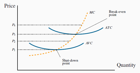
But how low can the price go before supply becomes unprofitable? To understand the supply decision further, in Figure 9.2 the firm’s AVC and ATC curves have been added to Figure 9.1.
A price below  does not cover variable costs, so the firm should
shut down. Between prices
does not cover variable costs, so the firm should
shut down. Between prices  and
and  , the producer can cover variable, but not total, costs and there should produce in the
short run if fixed costs are ‘sunk’. In the long-run the firm must close if the price does not reach
, the producer can cover variable, but not total, costs and there should produce in the
short run if fixed costs are ‘sunk’. In the long-run the firm must close if the price does not reach  . Profits are made if the price exceeds
  . The short-run supply curve is the quantity supplied at each price. It is therefore the MC curve above
  .
.
First, note that any price below  , which corresponds to the minimum
of the ATC curve, yields no profit, since it does not enable the producer to cover all of his costs. This price is therefore called the break-even price. Second, any price below
, which corresponds to the minimum
of the ATC curve, yields no profit, since it does not enable the producer to cover all of his costs. This price is therefore called the break-even price. Second, any price below  , which corresponds to the minimum of the AVC, does not even enable the producer to
cover variable costs. What about a price such as
, which corresponds to the minimum of the AVC, does not even enable the producer to
cover variable costs. What about a price such as  , that lies between
these? The answer is that, if the supplier has already incurred some fixed costs, he should continue to produce, provided he can cover his variable cost. But in the long run he must cover all
of his costs, fixed and variable. Therefore, if the price falls below
, that lies between
these? The answer is that, if the supplier has already incurred some fixed costs, he should continue to produce, provided he can cover his variable cost. But in the long run he must cover all
of his costs, fixed and variable. Therefore, if the price falls below  , he should shut down, even in the short run. This price is therefore called the shut-down price. If a price at least equal
to
, he should shut down, even in the short run. This price is therefore called the shut-down price. If a price at least equal
to  cannot be sustained in the long run, he should leave the
industry. But at a price such as P2 he can cover variable costs and therefore should continue to produce in the short run. The firm’s short-run supply curve is, therefore, that portion of the
MC curve above the minimum of the AVC.
cannot be sustained in the long run, he should leave the
industry. But at a price such as P2 he can cover variable costs and therefore should continue to produce in the short run. The firm’s short-run supply curve is, therefore, that portion of the
MC curve above the minimum of the AVC.
To illustrate this more concretely, let’s go back to the example of our snowboard producer, and imagine that he is producing in a perfectly competitive marketplace. How should he behave in response to different prices? Table 9.1 reproduces the data from Table 8.2.
| Labour | Output | Total Revenue $ | Average Variable Cost | Average Total Cost $ | Marginal Cost $ | Total Cost $ | Production Decision |
| L | Q | TR | AVC | ATC | MC | TC | No production where P < min AVC |
| 0 | 0 | ||||||
| 1 | 15 | 1,050 | 66.7 | 266.7 | 266.7 | 4,000 | |
| 2 | 40 | 2,800 | 50.0 | 125.0 | 40.0 | 5,000 | |
| 3 | 70 | 4,900 | 42.9 | 85.7 | 33.3 | 6,000 | |
| 4 | 110 | 7,700 | 36.4 | 63.6 | 25.0 | 7,000 | |
| 5 | 145 | 10,150 | 34.5 | 55.2 | 28.6 | 8,000 | |
| 6 | 175 | 12,250 | 34.3 | 51.4 | 33.3 | 9,000 | Min AVC |
| 7 | 200 | 14,000 | 35.0 | 50.0 | 40.0 | 10,000 | Price covers AVC, not ATC |
| 8 | 220 | 15,400 | 36.4 | 50.0 | 50.0 | 11,000 | Profit where P > min ATC, and supply where P = MC |
| 9 | 235 | 16,450 | 38.3 | 51.1 | 66.7 | 12,000 | |
| 10 | 240 | 16,800 | 41.7 | 54.2 | 200.0 | 13,000 |
Output Price=$70; Wage=$1,000; Fixed Cost=$3,000
The shut-down price corresponds to the minimum
value of the AVC curve.
The break-even price corresponds to the minimum of
the ATC curve.
The firm’s short-run supply curve is that portion
of the MC curve above the minimum of the AVC.
Suppose that the price is $70. How many boards should he produce? The answer is defined by the behaviour of the MC curve. For any output less than or equal to 235, the MC is less than the price. For example, at L = 9 and Q = 235, the MC is $66.7. At this output level, he makes a profit on the marginal unit produced, because the MC is less than the revenue he gets from selling it.
But, at outputs above this, he registers a loss on the marginal units because the MC exceeds the revenue. For example, at L = 10 and Q = 240, the MC is $200. Clearly, 235 snowboards is the optimum. To produce more would generate a loss on each additional unit, because the additional cost would exceed the additional revenue. Furthermore, to produce fewer snowboards would mean not availing of the potential for profit on additional boards.
His profit is based on the difference between revenue per unit and cost per unit at this output: (P - ATC). Since the ATC for the 235 units produced by the nine workers is $51.1, his profit margin is $70 - $51.1 = $18.9 per board, and total profit is therefore 235 X $18.9 = $4441.5.
Let us establish two other key outputs and prices for the producer. First, the shut-down point is the minimum of his AVC curve. Table 9.1 tells us that the price must be at least $34.3 for him to be willing to supply any output, since that is the value of the AVC at its minimum. Second, the minimum of his ATC is at $50. Accordingly, provided the price exceeds $50, he will cover both variable and fixed costs and make a maximum profit when he chooses an output where P = MC, above P=$50. Finally we can specify the short run supply curve for Black Diamond Snowboards: it is the segment of the MC curve in Figure 8.4 above the AVC curve.
Given that we have developed the individual firm’s supply curve, the next task is to develop the industry supply curve.
- 3697 reads
