


When aggregating the firm-level supply curves, as illustrated in Figure 9.3, we did not assume that all firms were identical. In that example, firm A has a cost structure with a lower AVC curve, since its supply curve starts at a lower dollar value. This indicates that firm A may have a larger plant size than firm B – one that puts A closer to the minimum efficient scale region of its long-run ATC curve.
Can firm B survive with his current scale of operation in the long run? Our industry dynamics indicate that it cannot. The reason is that, provided some firms are making economic profits, new entrepreneurs will enter the industry and drive the price down to the minimum of the ATC curve of those firms who are operating with the lowest cost plant size. B-type firms will therefore be forced either to leave the industry or to adjust to the least-cost plant size—corresponding to the lowest point on its long-run ATC curve. Remember that the same technology is available to all firms; they each have the same long-run ATC curve, and may choose different scales of operation in the short run, as illustrated in Figure 9.7. But in the long run they must all produce using the minimum-cost plant size, or else they will be driven from the market.
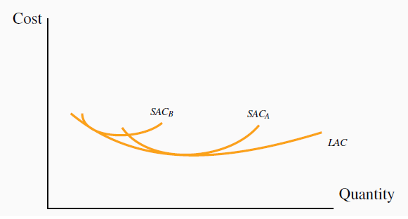
Firm B cannot compete with Firm A in the long run given that B has a less efficient plant size than firm A. The equilibrium long-run price equals the minimum of the LAC. At this price firm B must move to a more efficient plant size or make losses.
This behaviour enables us to define a long-run industry supply. The long run involves the entry and exit of firms, and leads to a price corresponding to the minimum of the long-run ATC curve. Therefore, if the long-run equilibrium price corresponds to this minimum, the long-run supply curve of the industry is defined by a particular price value—it is horizontal at that price. More or less output is produced as a result of firms entering or leaving the industry, with those present always producing at the same unit cost in a long-run equilibrium.
 Industry supply in the long-run in perfect
competition is horizontal at a price corresponding to the minimum of the representative firm’s long-run ATC curve.
Industry supply in the long-run in perfect
competition is horizontal at a price corresponding to the minimum of the representative firm’s long-run ATC curve.
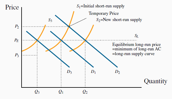
This industry’s long-run supply curve,  , and a particular short-run
supply are illustrated in Figure 9.8.
Different points on
, and a particular short-run
supply are illustrated in Figure 9.8.
Different points on  are attained when demand shifts. Suppose that,
from an initial equilibrium Q
are attained when demand shifts. Suppose that,
from an initial equilibrium Q , defined by the intersection of
D
, defined by the intersection of
D and S
and S , demand increases from D
 to D
to D because of a growth in income. With a fixed number of firms, the additional demand can be met only at a higher price, where each existing firm produces more using their existing plant size. The
economic profits that result induce new operators to produce. This addition to the industry’s production capacity shifts the short-run supply outwards and price declines until normal profits
are once again being made. The new long-run equilibrium is at Q
because of a growth in income. With a fixed number of firms, the additional demand can be met only at a higher price, where each existing firm produces more using their existing plant size. The
economic profits that result induce new operators to produce. This addition to the industry’s production capacity shifts the short-run supply outwards and price declines until normal profits
are once again being made. The new long-run equilibrium is at Q , with
more firms each producing at the minimum of their long-run ATC curve,
, with
more firms each producing at the minimum of their long-run ATC curve,  .
.
The LR equilibrium price  is disturbed by a shift in demand from
D
is disturbed by a shift in demand from
D to D
to D . With a fixed number of firms,
  results. Profits accrue at this price and entry occurs. Therefore the SR supply shifts outwards until these profits are eroded and
the new equilibrium output is
results. Profits accrue at this price and entry occurs. Therefore the SR supply shifts outwards until these profits are eroded and
the new equilibrium output is  . If, instead, D falls
to
. If, instead, D falls
to  then firms exit because they make losses, S shifts back
until the price is driven up sufficiently to restore normal profits. With different outputs supplied in the long run at the same price
then firms exit because they make losses, S shifts back
until the price is driven up sufficiently to restore normal profits. With different outputs supplied in the long run at the same price  , therefore the long-run supply is horizontal at
  .
.
The same dynamic would describe the industry reaction to a decline in demand—price would fall, some firms would exit, and the resulting contraction in supply would force the price back up to
the long-run equilibrium level. This is illustrated by a decline in demand from D to  .
.
- 2633 reads
