


Table 12.1 contains
information from the example developed in Production and
cost. It can be used to illustrate how a firm reacts in the short run to a change in an input price. Such a response constitutes a demand function – a schedule relating the quantity
demanded for an input to different input prices. The output produced by the various numbers of workers yields a marginal product curve, whose values are stated in column 3. The marginal product
of labour,  , as developed in Production and cost, is the additional output resulting from one more worker being
employed, while holding constant the other (fixed) factors. But what is the dollar value to the firm of an additional worker? It is the additional value of output resulting from the additional
employee – the price of the output times the worker’s marginal contribution to output, his MP. We term this the value of the marginal product.
, as developed in Production and cost, is the additional output resulting from one more worker being
employed, while holding constant the other (fixed) factors. But what is the dollar value to the firm of an additional worker? It is the additional value of output resulting from the additional
employee – the price of the output times the worker’s marginal contribution to output, his MP. We term this the value of the marginal product.
| Workers | Output | MPL | VMPL = MPL X P | Marginal profit = (VMPL - wage) |
| (1) | (2) | (3) | (4) | (5) |
| 0 | 0 | |||
| 1 | 15 | 15 | 1050 | 150 |
| 2 | 40 | 25 | 1750 | 750 |
| 3 | 70 | 30 | 2100 | 1100 |
| 4 | 110 | 40 | 2800 | 1800 |
| 5 | 145 | 35 | 2450 | 1450 |
| 6 | 175 | 30 | 2100 | 1100 |
| 7 | 200 | 25 | 1750 | 750 |
| 8 | 220 | 20 | 1400 | 400 |
| 9 | 235 | 15 | 1050 | 50 |
| 10 | 240 | 5 | 350 | negative |
Each unit of labour costs $1000; output sells at a fixed price of $70 per unit
 The value of the marginal product is the marginal
product multiplied by the price of the good produced.
The value of the marginal product is the marginal
product multiplied by the price of the good produced.
In this example the  first rises and then falls. With each unit of
output selling for $70 the value of the marginal product of labour (
first rises and then falls. With each unit of
output selling for $70 the value of the marginal product of labour ( ) is given in column 4. The first worker produces 15 units each week, and since each unit sells for a price of $70, then his net
value to the firm is $1,500. A second worker produces 25 units, so his weekly value to the firm is $1,750, and so forth. If the weekly wage of each worker is $1,000 then the firm can estimate
its marginal profit from hiring each additional worker. This is given in the final column.
) is given in column 4. The first worker produces 15 units each week, and since each unit sells for a price of $70, then his net
value to the firm is $1,500. A second worker produces 25 units, so his weekly value to the firm is $1,750, and so forth. If the weekly wage of each worker is $1,000 then the firm can estimate
its marginal profit from hiring each additional worker. This is given in the final column.
It is profitable to hire more workers as long as the cost of an extra worker is less than the  . The equilibrium amount of labour to employ is therefore 9 units in this example. If the firm were to hire one more worker the
contribution of that worker to its profit would be negative, and if it hired one worker less it would forego the opportunity to make an additional profit of $50 on the 9th unit.
. The equilibrium amount of labour to employ is therefore 9 units in this example. If the firm were to hire one more worker the
contribution of that worker to its profit would be negative, and if it hired one worker less it would forego the opportunity to make an additional profit of $50 on the 9th unit.
Profit maximizing hiring rule:
- If the
 of next worker > wage, hire more labour.
- If the
 < wage, hire less labour.
To this point we have determined the profit maximizing amount of labour to employ when the output price and the wage are given. However, a demand function for labour reflects the demand for
labour at many different wage rates. Accordingly, suppose the wage rate is $1,500 per weekrather than $1,000. The optimal amount of labour to employ in this case is determined in exactly the
same manner: employ the amount of labour where its contribution is marginally profitable. Clearly the optimal amount to employ is 7 units: the value of the seventh worker to the firm is $1,750
and the value of the eighth worker is $1,400. Hence it would not be profitable to employ the eighth, because his marginal contribution to profit would be negative. Following the same procedure
we could determine the optimal labour to employ at any wage. It is evident that the  function is the demand for labour function because it determines the most profitable amount of labour to employ at any wage.
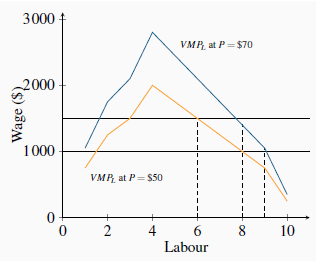
The optimal amount of labour to hire is illustrated in Figure 12.1. The wage and  curves come
from Table 12.1. The
curves come
from Table 12.1. The  curve has an upward sloping segment, reflecting increasing productivity, and then a
regular downward slope as developed in Production and cost.
At employment levels where the
curve has an upward sloping segment, reflecting increasing productivity, and then a
regular downward slope as developed in Production and cost.
At employment levels where the  is greater than the wage
additional labour should be employed. But when the
is greater than the wage
additional labour should be employed. But when the  falls below
the wage rate employment should stop. If labour is divisible into very small units, the optimal employment decision is where the
falls below
the wage rate employment should stop. If labour is divisible into very small units, the optimal employment decision is where the  function intersects the wage line.
The optimal hiring decision is defined by the condition that the value of the  is greater than or equal to the wage paid.
Figure 12.1 also illustrates what happens to hiring when the output price changes. Consider a reduction in its price to $50 from $70. The profit impact of such a change is negative because the value of each worker’s output has declined. Accordingly the demand curve must reflect this by shifting inward, as in the figure. At various wage rates, less labour is now demanded.
In this example the firm is a perfect competitor in the output market – the price of the good being produced is fixed. Where the firm is not a perfect competitor it faces a declining MR
function. In this case the value of the  is the product of MR and
 rather than P and
  . To distinguish the different output markets we use the term marginal revenue product of
labour (MRPL) when the demand for the output slopes downward. But the optimizing principle remains the same: the firm should calculate the value of each additional unit of labour, and hire up
to the point where the additional revenue produced by the worker exceeds or equals the additional cost of that worker.
. To distinguish the different output markets we use the term marginal revenue product of
labour (MRPL) when the demand for the output slopes downward. But the optimizing principle remains the same: the firm should calculate the value of each additional unit of labour, and hire up
to the point where the additional revenue produced by the worker exceeds or equals the additional cost of that worker.
The marginal revenue product of labour is the
additional revenue generated by hiring one more unit of labour where the marginal revenue declines.
- 3341 reads
