


Panel (d) of Figure Figure 3.14 shows that a decrease in supply shifts the supply curve to the left. The equilibrium price rises to $7 per pound. As the price rises to the new equilibrium level, the quantity demanded decreases to 20 million pounds of coffee per month.
Possible supply shifters that could reduce supply include an increase in the prices of inputs used in the production of coffee, an increase in the returns available from alternative uses of these inputs, a decline in production because of problems in technology (perhaps caused by a restriction on pesticides used to protect coffee beans), a reduction in the number of coffee-producing firms, or a natural event, such as excessive rain.
Heads Up!
You are likely to be given problems in which you will have to shift a demand or supply curve.
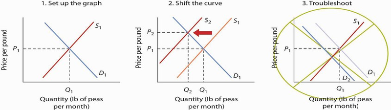
Suppose you are told that an invasion of pod-crunching insects has gobbled up half the crop of fresh peas, and you are asked to use demand and supply analysis to predict what will happen to the price and quantity of peas demanded and supplied. Here are some suggestions.
Put the quantity of the good you are asked to analyze on the horizontal axis and its price on the vertical axis. Draw a downward-sloping line for demand and an upward-sloping line for supply. The initial equilibrium price is determined by the intersection of the two curves. Label the equilibrium solution. You may find it helpful to use a number for the equilibrium price instead of the letter “P.” Pick a price that seems plausible, say, 79¢ per pound. Do not worry about the precise positions of the demand and supply curves; you cannot be expected to know what they are.
Step 2 can be the most difficult step; the problem is to decide which curve to shift. The key is to remember the difference between a change in demand or supply and a change in quantity demanded or supplied. At each price, ask yourself whether the given event would change the quantity demanded. Would the fact that a bug has attacked the pea crop change the quantity demanded at a price of, say, 79¢ per pound? Clearly not; none of the demand shifters have changed. The event would, however, reduce the quantity supplied at this price, and the supply curve would shift to the left. There is a change in supply and a reduction in the quantity demanded.
There is no change in demand.
Next check to see whether the result you have obtained makes sense. The graph in Step 2 makes sense; it shows price rising and quantity demanded falling.
It is easy to make a mistake such as the one shown in the third figure of this Heads Up! One might, for example, reason that when fewer peas are available, fewer will be demanded, and therefore the demand curve will shift to the left. This suggests the price of peas will fall—but that does not make sense. If only half as many fresh peas were available, their price would surely rise. The error here lies in confusing a change in quantity demanded with a change in demand. Yes, buyers will end up buying fewer peas. But no, they will not demand fewer peas at each price than before; the demand curve does not shift.
Simultaneous Shifts
As we have seen, when either the demand or the supply curve shifts, the results are unambiguous; that is, we know what will happen to both equilibrium price and equilibrium quantity, so long as we know whether demand or supply increased or decreased. However, in practice, several events may occur at around the same time that cause both the demand and supply curves to shift. To figure out what happens to equilibrium price and equilibrium quantity, we must know not only in which direction the demand and supply curves have shifted but also the relative amount by which each curve shifts. Of course, the demand and supply curves could shift in the same direction or in opposite directions, depending on the specific events causing them to shift.
For example, all three panels of Figure Figure 3.16 show a decrease in demand for coffee (caused perhaps by a decrease in the price of a substitute good, such as tea) and a simultaneous decrease in the supply of coffee (caused perhaps by bad weather). Since reductions in demand and supply, considered separately, each cause the equilibrium quantity to fall, the impact of both curves shifting simultaneously to the left means that the new equilibrium quantity of coffee is less than the old equilibrium quantity. The effect on the equilibrium price, though, is ambiguous. Whether the equilibrium price is higher, lower, or unchanged depends on the extent to which each curve shifts.
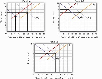
Both the demand and the supply of coffee decrease. Since decreases in demand and supply, considered separately, each cause equilibrium quantity to fall, the impact of both decreasing simultaneously means that a new equilibrium quantity of coffee must be less than the old equilibrium quantity. In Panel (a), the demand curve shifts farther to the left than does the supply curve, so equilibrium price falls. In Panel (b), the supply curve shifts farther to the left than does the demand curve, so the equilibrium price rises. In Panel (c), both curves shift to the left by the same amount, so equilibrium price stays the same.
If the demand curve shifts farther to the left than does the supply curve, as shown in Panel (a) of Figure 3.16, then the equilibrium price will be lower than it was before the curves shifted. In this case the new equilibrium price falls from $6 per pound to $5 per pound. If the shift to the left of the supply curve is greater than that of the demand curve, the equilibrium price will be higher than it was before, as shown in Panel (b). In this case, the new equilibrium price rises to $7 per pound. In Panel (c), since both curves shift to the left by the same amount, equilibrium price does not change; it remains $6 per pound.
Regardless of the scenario, changes in equilibrium price and equilibrium quantity resulting from two different events need to be considered separately. If both events cause equilibrium price or quantity to move in the same direction, then clearly price or quantity can be expected to move in that direction. If one event causes price or quantity to rise while the other causes it to fall, the extent by which each curve shifts is critical to figuring out what happens. Figure 3.17 summarizes what may happen to equilibrium price and quantity when demand and supply both shift.
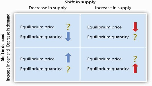
If simultaneous shifts in demand and supply cause equilibrium price or quantity to move in the same direction, then equilibrium price or quantity clearly moves in that direction. If the shift in one of the curves causes equilibrium price or quantity to rise while the shift in the other curve causes equilibrium price or quantity to fall, then the relative amount by which each curve shifts is critical to figuring out what happens to that variable.
As demand and supply curves shift, prices adjust to maintain a balance between the quantity of a good demanded and the quantity supplied. If prices did not adjust, this balance could not be maintained.
Notice that the demand and supply curves that we have examined in this chapter have all been drawn as linear. This simplification of the real world makes the graphs a bit easier to read without sacrificing the essential point: whether the curves are linear or nonlinear, demand curves are downward sloping and supply curves are generally upward sloping. As circumstances that shift the demand curve or the supply curve change, we can analyze what will happen to price and what will happen to quantity.
- 3859 reads
