


What happens to the price elasticity of demand when we travel along the demand curve? The answer depends on the nature of the demand curve itself. On a linear demand curve, such as the one in Figure 5.2, elasticity becomes smaller (in absolute value) as we travel downward and to the right.
The price elasticity of demand varies between different pairs of points along a linear demand curve. The lower the price and the greater the quantity demanded, the lower the absolute value of the price elasticity of demand.
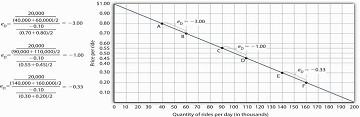
Figure 5.2 shows the same demand curve we saw in Figure 5.1. We have already calculated the priceelasticity of demand between points A and B; it equals −3.00. Notice, however, that when we use thesame method to compute the price elasticity of demand between other sets of points, our answer varies.For each of the pairs of points shown, the changes in price and quantity demanded are the same (a$0.10 decrease in price and 20,000 additional rides per day, respectively). But at the high prices and lowquantities on the upper part of the demand curve, the percentage change in quantity is relatively large,whereas the percentage change in price is relatively small. The absolute value of the price elasticity of demand is thus relatively large. As we move down the demand curve, equal changes in quantity represent smaller and smaller percentage changes, whereas equal changes in price represent larger and larger percentage changes, and the absolute value of the elasticity measure declines. Between points C and D,for example, the price elasticity of demand is −1.00, and between points E and F the price elasticity of demand is −0.33.
On a linear demand curve, the price elasticity of demand varies depending on the interval over which we are measuring it. For any linear demand curve, the absolute value of the price elasticity of demand will fall as we move down and to the right along the curve.
The Price Elasticity of Demand and Changes in Total Revenue
Suppose the public transit authority is considering raising fares. Will its total revenues go up or down? Total revenue is the price per unit times the number of units sold. In this case, it is the fare timesthe number of riders. The transit authority will certainly want to know whether a price increase willcause its total revenue to rise or fall. In fact, determining the impact of a price change on total revenueis crucial to the analysis of many problems in economics.
We will do two quick calculations before generalizing the principle involved. Given the demandcurve shown in Figure 5.2, we see that at a price of $0.80, the transit authority will sell 40,000 rides per day. Total revenue would be $32,000 per day ($0.80 times 40,000). If the price were lowered by $0.10 to $0.70, quantity demanded would increase to 60,000 rides and total revenue would increase to $42,000($0.70 times 60,000). The reduction in fare increases total revenue. However, if the initial price hadbeen $0.30 and the transit authority reduced it by $0.10 to $0.20, total revenue would decrease from$42,000 ($0.30 times 140,000) to $32,000 ($0.20 times 160,000). So it appears that the impact of a pricechange on total revenue depends on the initial price and, by implication, the original elasticity. Wegeneralize this point in the remainder of this section.
The problem in assessing the impact of a price change on total revenue of a good or service is thata change in price always changes the quantity demanded in the opposite direction. An increase in price reduces the quantity demanded, and a reduction in price increases the quantity demanded. The question is how much. Because total revenue is found by multiplying the price per unit times the quantity demanded, it is not clear whether a change in price will cause total revenue to rise or fall.
We have already made this point in the context of the transit authority. Consider the following three examples of price increases for gasoline, pizza, and diet cola.
Suppose that 1,000 gallons of gasoline per day are demanded at a price of $4.00 per gallon. Totalrevenue for gasoline thus equals $4,000 per day (=1,000 gallons per day times $4.00 per gallon). If an increase in the price of gasoline to $4.25 reduces the quantity demanded to 950 gallons per day, totalrevenue rises to $4,037.50 per day (=950 gallons per day times $4.25 per gallon). Even though people consume less gasoline at $4.25 than at $4.00, total revenue rises because the higher price more than makes up for the drop in consumption.
Next consider pizza. Suppose 1,000 pizzas per week are demanded at a price of $9 per pizza. Totalrevenue for pizza equals $9,000 per week (=1,000 pizzas per week times $9 per pizza). If an increase in the price of pizza to $10 per pizza reduces quantity demanded to 900 pizzas per week, total revenue willstill be $9,000 per week (=900 pizzas per week times $10 per pizza). Again, when price goes up, consumers buy less, but this time there is no change in total revenue.
Now consider diet cola. Suppose 1,000 cans of diet cola per day are demanded at a price of $0.50 per can. Total revenue for diet cola equals $500 per day (=1,000 cans per day times $0.50 per can). If an increase in the price of diet cola to $0.55 per can reduces quantity demanded to 880 cans per month, total revenue for diet cola falls to $484 per day (=880 cans per day times $0.55 per can). As in the case of gasoline, people will buy less diet cola when the price rises from $0.50 to $0.55, but in this example total revenue drops. In our first example, an increase in price increased total revenue. In the second, a price increase left total revenue unchanged. In the third example, the price rise reduced total revenue. Is there a way to predict how a price change will affect total revenue? There is; the effect depends on the price elasticity of demand.
- 43753 reads
