


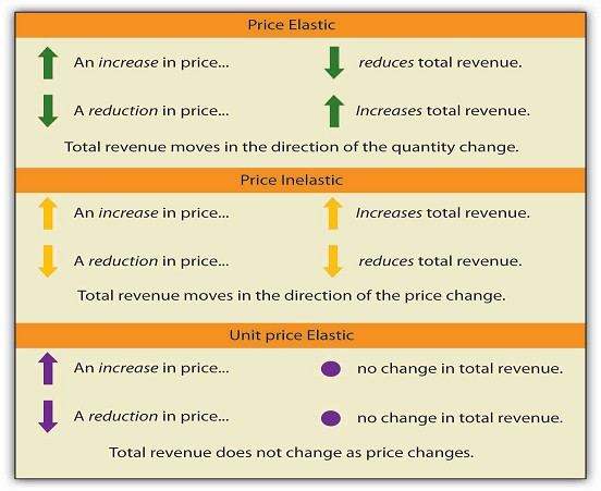
When the price of a good or service changes, the quantity demanded changes in the opposite direction.Total revenue will move in the direction of the variable that changes by the larger percentage. If the variables move by the same percentage, total revenue stays the same. If quantity demanded changes by a larger percentage than price (i.e., if demand is price elastic), total revenue will change in the direction of the quantity change. If price changes by a larger percentage than quantity demanded (i.e., if demand is price inelastic), total revenue will move in the direction of the price change. If price and quantity demanded change by the same percentage (i.e., if demand is unit price elastic), then total revenue doesnot change.
When demand is price inelastic, a given percentage change in price results in a smaller percentage change in quantity demanded. That implies that total revenue will move in the direction of the price change: a reduction in price will reduce total revenue, and an increase in price will increase it.
Consider the price elasticity of demand for gasoline. In the example above, 1,000 gallons of gasoline were purchased each day at a price of $4.00 per gallon; an increase in price to $4.25 per gallon reduced the quantity demanded to 950 gallons per day. We thus had an average quantity of 975 gallons per day and an average price of $4.125. We can thus calculate the arc price elasticity of demand for gasoline:
Percentage change in quantity demanded = −50 / 975 = −5.1%
Percentage change in price = 0.25 / 4.125=6.06%
Price elasticity of demand = −5.1% / 6.06% = −0.84
The demand for gasoline is price inelastic, and total revenue moves in the direction of the price change.When price rises, total revenue rises. Recall that in our example above, total spending on gasoline(which equals total revenues to sellers) rose from $4,000 per day (=1,000 gallons per day times $4.00) to $4037.50 per day (=950 gallons per day times $4.25 per gallon).
When demand is price inelastic, a given percentage change in price results in a smaller percentage change in quantity demanded. That implies that total revenue will move in the direction of the price change: an increase in price will increase total revenue, and a reduction in price will reduce it.
Consider again the example of pizza that we examined above. At a price of $9 per pizza, 1,000 pizzas per week were demanded. Total revenue was $9,000 per week (=1,000 pizzas per week times $9 per pizza). When the price rose to $10, the quantity demanded fell to 900 pizzas per week. Total revenue remained $9,000 per week (=900 pizzas per week times $10 per pizza). Again, we have an average quantity of 950 pizzas per week and an average price of $9.50. Using the arc elasticity method, we can compute:
Percentage change in quantity demanded = − 100 / 950 = − 10.5%
Percentage change in price = $1.00 / $9.50 = 10.5%
Price elasticity of demand = − 10.5% / 10.5% = − 1.0
Demand is unit price elastic, and total revenue remains unchanged. Quantity demanded falls by the same percentage by which price increases.
Consider next the example of diet cola demand. At a price of $0.50 per can, 1,000 cans of diet cola were purchased each day. Total revenue was thus $500 per day (=$0.50 per can times 1,000 cans per day). An increase in price to $0.55 reduced the quantity demanded to 880 cans per day. We thus havean average quantity of 940 cans per day and an average price of $0.525 per can. Computing the price elasticity of demand for diet cola in this example, we have:
Percentage change in quantity demanded = − 120 / 940 = − 12.8%
Percentage change in price = $0.05 / $0.525 = 9.5%
Price elasticity of demand = − 12.8% / 9.5% = − 1.3
The demand for diet cola is price elastic, so total revenue moves in the direction of the quantity change.It falls from $500 per day before the price increase to $484 per day after the price increase.
A demand curve can also be used to show changes in total revenue. Figure 5.3 shows the demandcurve from Figure 5.1 and Figure 5.2. At point A, total revenue from public transit rides is given by the area of a rectangle drawn with point A in the upper right-hand corner and the origin in the lower left- hand corner. The height of the rectangle is price; its width is quantity. We have already seen that total revenue at point A is $32,000 ($0.80 × 40,000). When we reduce the price and move to point B, the rectangle showing total revenue becomes shorter and wider. Notice that the area gained in moving to the rectangle at B is greater than the area lost; total revenue rises to $42,000 ($0.70 × 60,000). Recall from Figure 5.2 that demand is elastic between points A and B. In general, demand is elastic in the upper half of any linear demand curve, so total revenue moves in the direction of the quantity change.
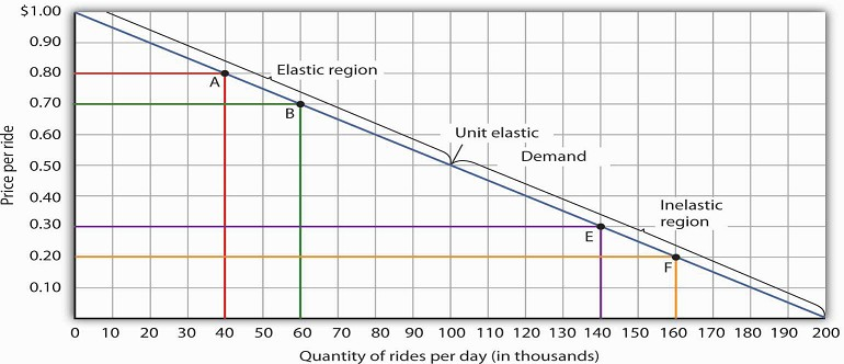
Moving from point A to point B implies a reduction in price and an increase in the quantity demanded. Demand iselastic between these two points. Total revenue, shown by the areas of the rectangles drawn from points A and B to the origin, rises. When we move from point E to point F, which is in the inelastic region of the demand curve, total revenue falls.
A movement from point E to point F also shows a reduction in price and an increase in quantity demanded. This time, however, we are in an inelastic region of the demand curve. Total revenue now moves in the direction of the price change—it falls. Notice that the rectangle drawn from point F is smaller in area than the rectangle drawn from point E, once again confirming our earlier calculation.
We have noted that a linear demand curve is more elastic where prices are relatively high and quantitiesrelatively low and less elastic where prices are relatively low and quantities relatively high. We can be even more specific. For any linear demand curve, demand will be price elastic in the upper half of the curve and price inelastic in its lower half. At the midpoint of a linear demand curve, demand is unit price elastic.
- 12849 reads
