


As we have already seen, a consumer’s choices are limited by the budget available. Total spending for goods and services can fall short of the budget constraint but may not exceed it.
Algebraically, we can write the budget constraint for two goods X and Y as:
EQUATION 7.7

where PX and PY are the prices of goods X and Y and QX and QY are the quantities of goods X andY chosen. The total income available to spend on the two goods is B, the consumer’s budget.
Equation 7.7 states that total expenditures on goods X and Y (the left-hand side of the equation) cannot exceed B.
Suppose a college student, Janet Bain, enjoys skiing and horseback riding. A day spent pursuingeither activity costs $50. Suppose she has $250 available to spend on these two activities each semester.Ms. Bain’s budget constraint is illustrated in Figure 7.7
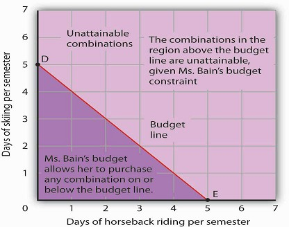
The budget line shows combinations of the skiing and horseback riding Janet Bain could consume if the price of each activity is $50 and she has $250 available for them each semester. The slope of this budget line is −1, the negative of the price of horseback riding divided by the price of skiing.
For a consumer who buys only two goods, the budget constraint can be shown with a budget line. Abudget line shows graphically the combinations of two goods a consumer can buy with a given budget.
The budget line shows all the combinations of skiing and horseback riding Ms. Bain can purchasewith her budget of $250. She could also spend less than $250, purchasing combinations that lie below and to the left of the budget line in Figure 7.7. Combinations above and to the right of the budget line are beyond the reach of her budget.
The vertical intercept of the budget line (point D) is given by the number of days of skiing permonth that Ms. Bain could enjoy, if she devoted all of her budget to skiing and none to horseback riding.She has $250, and the price of a day of skiing is $50. If she spent the entire amount on skiing, she could ski 5 days per semester. She would be meeting her budget constraint, since:
$50 × 0 + $50 × 5 = $250
The horizontal intercept of the budget line (point E) is the number of days she could spend horseback riding if she devoted her $250 entirely to that sport. She could purchase 5 days of either skiing or horseback riding per semester. Again, this is within her budget constraint, since:
$50 × 5 + $50 × 0 = $250
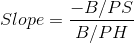
Because the budget line is linear, we can compute its slope between any two points. Between points Dand E the vertical change is −5 days of skiing; the horizontal change is 5 days of horseback riding. The slope is thus − 5 / 5 = − 1 . More generally, we find the slope of the budget line by finding the vertical and horizontal intercepts and then computing the slope between those two points. The vertical intercept of the budget line is found by dividing Ms. Bain’s budget, B, by the price of skiing, the good on the vertical axis (PS). The horizontal intercept is found by dividing B by the price of horseback riding, the good on the horizontal axis (PH). The slope is thus:
EQUATION 7.8
Simplifying this equation, we obtain
EQUATION 7.9
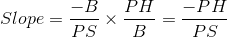
After canceling, Equation 7.9 shows that the slope of a budget line is the negative of the price of the good on the horizontal axis divided by the price of the good on the vertical axis.
Heads Up!
It is easy to go awry on the issue of the slope of the budget line: It is the negative of the price of the good on the horizontal axis divided by the price of the good on the vertical axis. But does not slope equal the change in the vertical axis divided by the change in the horizontal axis? The answer, of course, is that the definition of slope has not changed. Notice that Equation 7.8 gives the vertical change divided by the horizontal change between two points. We then manipulated Equation 7.8 a bit to get to Equation 7.9 and found that slope also equaled the negative of the price of the good on the horizontal axis divided by the price of the good on the vertical axis. Price is not the variable that is shown on the two axes. The axes show the quantities of the two goods.
- 2028 reads
