


Suppose Ms. Bain spends 2 days skiing and 3 days horseback riding per semester. She will derive some level of total utility from that combination of the two activities. There are other combinations of the two activities that would yield the same level of total utility. Combinations of two goods that yield equal levels of utility are shown on an indifference curve. 1 Because all points along an indifference curve generate the same level of utility, economists say that a consumer is indifferent between them.
Figure 7.8 shows an indifference curve for combinations of skiing and horseback riding that yieldthe same level of total utility. Point X marks Ms. Bain’s initial combination of 2 days skiing and 3 days horseback riding per semester. The indifference curve shows that she could obtain the same level ofutility by moving to point W, skiing for 7 days and going horseback riding for 1 day. She could also get the same level of utility at point Y, skiing just 1 day and spending 5 days horseback riding. Ms. Bain isindifferent among combinations W, X, and Y. We assume that the two goods are divisible, so she is indifferent between any two points along an indifference curve.
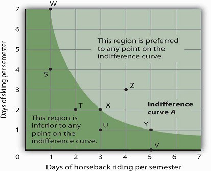
The indifference curve A shown here gives combinations of skiing and horseback riding that produce the samelevel of utility. Janet Bain is thus indifferent to which point on the curve she selects. Any point below and to the left of the indifference curve would produce a lower level of utility; any point above and to the right of the indifference curve would produce a higher level of utility.
Now look at point T in Figure 7.8. It has the same amount of skiing as point X, but fewer days arespent horseback riding. Ms. Bain would thus prefer point X to point T. Similarly, she prefers X to U.What about a choice between the combinations at point W and point T? Because combinations X andW are equally satisfactory, and because Ms. Bain prefers X to T, she must prefer W to T. In general, any combination of two goods that lies below and to the left of an indifference curve for those goods yields less utility than any combination on the indifference curve. Such combinations are inferior to combinations on the indifference curve.
Point Z, with 3 days of skiing and 4 days of horseback riding, provides more of both activities thanpoint X; Z therefore yields a higher level of utility. It is also superior to point W. In general, any combination that lies above and to the right of an indifference curve is preferred to any point on the indifference curve.
We can draw an indifference curve through any combination of two goods. Figure 7.9shows indifferencecurves drawn through each of the points we have discussed. Indifference curve A from Figure 7.8 is inferior to indifference curve B. Ms. Bain prefers all the combinations on indifference curve B to those on curve A, and she regards each of the combinations on indifference curve C as inferior to those on curves A and B.
Although only three indifference curves are shown in Figure 7.9, in principle an infinite numbercould be drawn. The collection of indifference curves for a consumer constitutes a kind of map illustrating a consumer’s preferences. Different consumers will have different maps. We have good reason to expect the indifference curves for all consumers to have the same basic shape as those shown here:They slope downward, and they become less steep as we travel down and to the right along them.
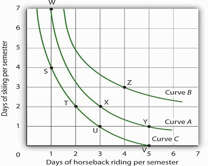
Each indifference curve suggests combinations among which the consumer is indifferent. Curves that are higherand to the right are preferred to those that are lower and to the left. Here, indifference curve B is preferred to curve A, which is preferred to curve C.
The slope of an indifference curve shows the rate at which two goods can be exchanged without affectingthe consumer’s utility. Figure 7.10 shows indifference curve C from Figure 7.9. Suppose Ms. Bain is at point S, consuming 4 days of skiing and 1 day of horseback riding per semester. Suppose she spends another day horseback riding. This additional day of horseback riding does not affect her utility if she gives up 2 days of skiing, moving to point T. She is thus willing to give up 2 days of skiing for asecond day of horseback riding. The curve shows, however, that she would be willing to give up at most 1 day of skiing to obtain a third day of horseback riding (shown by point U).
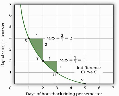
The marginal rate of substitution is equal to the absolute value of the slope of an indifference curve. It is themaximum amount of one good a consumer is willing to give up to obtain an additional unit of another. Here, it is the number of days of skiing Janet Bain would be willing to give up to obtain an additional day of horseback riding.Notice that the marginal rate of substitution (MRS) declines as she consumes more and more days of horseback riding.
The maximum amount of one good a consumer would be willing to give up in order to obtain an additionalunit of another is called the marginal rate of substitution (MRS), which is equal to the absolute value of the slope of the indifference curve between two points. Figure 7.10 shows that as Ms. Baindevotes more and more time to horseback riding, the rate at which she is willing to give up days of skiing for additional days of horseback riding—her marginal rate of substitution—diminishes.
- 4440 reads
