


Although the points plotted in Figure 31.3 are not consistent with a Phillips curve, we can find a relationship. Suppose we draw connecting lines through the sequence of observations, as is done in Figure 31.4. This approach suggests a pattern of clockwise loops, at least until 2002 when we see the beginnings of a counterclockwise loop. We see periods in which inflation rises as unemployment falls, followed by periods in which unemployment rises while inflation remains high or fairly constant. And those periods are followed by periods in which inflation and unemployment both fall.
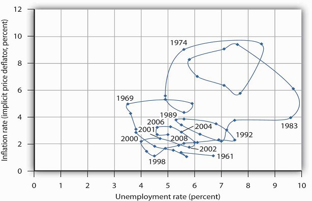
Sources: Economic Report of the President, 2009, Tables B-3 and B-42; data for 2008 are from the Bureau of Economic Analysis, Table 1.14 (revised March 26, 2009) and the Bureau of Labor Statistics (extracted April 14, 2009).
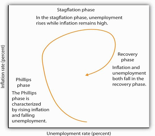
Figure 31.5 gives an idealized version of the general cycle suggested by the data in Figure 31.4. There is a Phillips phase in which inflation rises as unemployment falls. In this phase, the relationship suggested by the Phillips curve holds. The Phillips phase is followed by a stagflation phase in which inflation remains high while unemployment increases. The term, coined by Massachusetts Institute of Technology economist and Nobel laureate Paul Samuelson during the 1970s, suggests a combination of a stagnating economy and continued inflation. And finally, there is a recovery phase in which inflation and unemployment both decline. This pattern of a Phillips phase, then stagflation, and then a recovery can be termed the inflation–unemployment cycle.
Trace the path of the inflation–unemployment cycle as it unfolds in Figure 31.4. Starting with the Phillips phase in the 1960s, we see that the economy went through three inflation–unemployment cycles through the 1970s. Each took the United States to successively higher rates of inflation and unemployment. As the cycle that began in the late 1970s passed through the stagflation phase, however, something quite significant happened. The economy suffered its highest rate of unemployment since the Great Depression during that period. It also achieved its most dramatic gains against inflation. Since then, fluctuations in inflation and unemployment have become less severe. The recovery phase of the 1990s was the longest since the U.S. government began tracking inflation and unemployment. Good luck explains some of that: oil prices fell in the late 1990s, shifting the short-run aggregate supply curve to the right. That boosted real GDP and put downward pressure on the price level. But one cause of that improved performance seemed to be the better understanding economists gained from some policy mistakes of the 1970s.
In the early 2000s, following the brief recession in 2001, the inflation– unemployment trajectory moves in a counterclockwise direction, as the economy moved back quickly into the Phillips phase of falling unemployment and rising inflation but at higher levels of both compared to what prevailed in the late 1990s. During this recent period, oil and other commodity prices were rising, due primarily to rising demand in developing countries, principally China and India. Thus, the short-run aggregate supply curve was moving to the left while aggregate demand was shifting to the right.
The next section will explain these experiences in a stylized way in terms of the aggregate demand and supply model.
KEY TAKEAWAYS
- The view that there is a trade-off between inflation and unemployment is expressed by a Phillips curve. While there are periods in which a trade-off between inflation and unemployment exists, the actual relationship between these variables between 1961 and 2002 followed a cyclical pattern: the inflation– unemployment cycle.
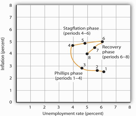
- In a Phillips phase, the inflation rate rises and unemployment falls. A stagflation phase is marked by rising unemployment while inflation remains high. In a recovery phase, inflation and unemployment both fall.
TRY IT!
Suppose an economy has experienced the rates of inflation and of unemployment shown below. Plot these data graphically in a grid with the inflation rate on the vertical axis and the unemployment rate on the horizontal axis. Identify the periods during which the economy experienced each of the three phases of the inflation– unemployment cycle identified in the text.
|
Period |
Unemployment rate (%) |
Inflation rate (%) |
|---|---|---|
|
1 |
2.5 |
6.3 |
|
2 |
2.6 |
5.9 |
|
3 |
2.8 |
4.8 |
|
4 |
4.7 |
4.1 |
|
5 |
4.9 |
5.0 |
|
6 |
5.0 |
6.1 |
|
7 |
4.5 |
5.7 |
|
8 |
4.0 |
5.1 |
Case in Point: Some Reflections on the 1970s
Looking back, we may find it difficult to appreciate how stunning the experience of 1970 and 1971 was. But those two years changed the face of macroeconomic thought.
Introductory textbooks of that time contained no mention of aggregate supply. The model of choice was the aggregate expenditures model. Students learned that the economy could be in
equilibrium below full employment, in which case unemployment would be the primary macroeconomic problem. Alternatively, equilibrium could occur at an income greater than the full employment
level, in which case inflation would be the main culprit to worry about.
These ideas could be summarized using a Phillips curve, a new analytical device. It suggested that economists could lay out for policy makers a menu of possibilities. Policy makers could then
choose the mix of inflation and unemployment they were willing to accept. Economists would then show them how to attain that mix with the appropriate fiscal and monetary policies.
Then 1970 and 1971 came crashing in on this well-ordered fantasy. President Richard Nixon had come to office with a pledge to bring down inflation. The consumer price index had risen 4.7%
during 1968, the highest rate since 1951. Mr. Nixon cut government purchases in 1969, and the Fed produced a sharp slowing in money growth. The president’s economic advisers predicted at the
beginning of 1970 that inflation and unemployment would both fall. Appraising the 1970 debacle early in 1971, the president’s economists said that the experience had not been consistent with
what standard models would predict. The economists suggested, however, that this was probably due to a number of transitory factors. Their forecast that inflation and unemployment would
improve in 1971 proved wide of the mark—the unemployment rate rose from 4.9% to 5.9% (an increase of 20%), while the rate of inflation measured by the change in the implicit price deflator
barely changed from 5.3% to 5.2%.
As we will see, the experience can be readily explained using the model of aggregate demand and aggregate supply. But this tool was not well developed then. The experience of the 1970s forced
economists back to their analytical drawing boards and spawned dramatic advances in our understanding of macroeconomic events. We will explore many of those advances in the next
chapter.
Source: Economic Report of the President, 1971, pp. 60–84.
ANSWER TO TRY IT! PROBLEM
- 4631 reads
