


Differences between groups or conditions are usually described in terms of the mean and standard deviation of each group or condition. For example, Thomas Ollendick and his colleagues conducted a study in which they evaluated two one-session treatments for simple phobias in children (Ollendick et al., 2009). 1They randomly assigned children with an intense fear (e.g., to dogs) to one of three conditions.
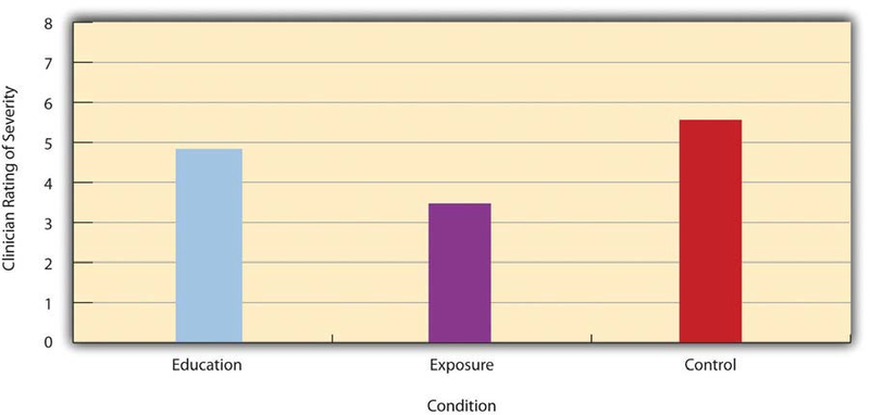
In the exposure condition, the children actually confronted the object of their fear under the guidance of a trained therapist. In the education condition, they learned about phobias and some strategies for coping with them. In the waitlist control condition, they were waiting to receive a treatment after the study was over. The severity of each child’s phobia was then rated on a 1-to-8 scale by a clinician who did not know which treatment the child had received. (This was one of several dependent variables.) The mean fear rating in the education condition was 4.83 with a standard deviation of 1.52, while the mean fear rating in the exposure condition was 3.47 with a standard deviation of 1.77. The mean fear rating in the control condition was 5.56 with a standard deviation of 1.21. In other words, both treatments worked, but the exposure treatment worked better than the education treatment. As we have seen, differences between group or condition means can be presented in a bar graph like that in Figure 12.5, where the heights of the bars represent the group or condition means. We will look more closely at creating American Psychological Association (APA)-style bar graphs shortly.
It is also important to be able to describe the strength of a statistical relationship, which is often referred to as the effect size. The most widely used measure of effect size for differences between group or condition means is called Cohen’s d, which is the difference between the two means divided by the standard deviation:
In this formula, it does not really matter which mean is  and
which is
and
which is  . If there is a treatment group and a control group, the
treatment group mean is usually
. If there is a treatment group and a control group, the
treatment group mean is usually  and the control group mean is
  . Otherwise, the larger mean is usually
  and the smaller mean
  so that Cohen’s d turns out to be positive. The standard deviation
in this formula is usually a kind of average of the two group standard deviations called the pooled-within groups standard deviation. To compute the pooled within-groups standard deviation, add
the sum of the squared differences for Group 1 to the sum of squared differences for Group 2, divide this by the sum of the two sample sizes, and then take the square root of that. Informally,
however, the standard deviation of either group can be used instead.
so that Cohen’s d turns out to be positive. The standard deviation
in this formula is usually a kind of average of the two group standard deviations called the pooled-within groups standard deviation. To compute the pooled within-groups standard deviation, add
the sum of the squared differences for Group 1 to the sum of squared differences for Group 2, divide this by the sum of the two sample sizes, and then take the square root of that. Informally,
however, the standard deviation of either group can be used instead.
Conceptually, Cohen’s dis the difference between the two means expressed in standard deviation units. (Notice its similarity to a zscore, which expresses the difference between an individual score and a mean in standard deviation units.) A Cohen’s dof 0.50 means that the two group means differ by 0.50 standard deviations (half a standard deviation). A Cohen’s dof 1.20 means that they differ by 1.20 standard deviations. But how should we interpret these values in terms of the strength of the relationship or the size of the difference between the means? Table 12.3 presents some guidelines for interpreting Cohen’s dvalues in psychological research (Cohen, 1992). 2 Values near 0.20 are considered small, values near 0.50 are considered medium, and values near 0.80 are considered large. Thus a Cohen’s d value of 0.50 represents a medium-sized difference between two means, and a Cohen’s dvalue of 1.20 represents a very large difference in the context of psychological research. In the research by Ollendick and his colleagues, there was a large difference (d= 0.82) between the exposure and education conditions.
|
Relationship strength |
Cohen’s d |
Pearson’s r |
|
Strong/large |
± 0.80 |
± 0.50 |
|
Medium |
± 0.50 |
± 0.30 |
|
Weak/small |
± 0.20 |
± 0.10 |
Cohen’s d is useful because it has the same meaning regardless of the variable being compared or the scale it was measured on. A Cohen’s d of 0.20 means that the two group means differ by 0.20 standard deviations whether we are talking about scores on the Rosenberg Self-Esteem scale, reaction time measured in milliseconds, number of siblings, or diastolic blood pressure measured in millimeters of mercury. Not only does this make it easier for researchers to communicate with each other about their results, it also makes it possible to combine and compare results across different studies using different measures.
Be aware that the term effect size can be misleading because it suggests a causal relationship—that the difference between the two means is an “effect” of being in one group or condition as opposed to another. Imagine, for example, a study showing that a group of exercisers is happier on average than a group of nonexercisers, with an “effect size” of d = 0.35. If the study was an experiment—with participants randomly assigned to exercise and no-exercise conditions—then one could conclude that exercising caused a small to medium-sized increase in happiness. If the study was correlational, however, then one could conclude only that the exercisers were happier than the nonexercisers by a small to medium-sized amount. In other words, simply calling the difference an “effect size” does not make the relationship a causal one.
Sex Differences Expressed as Cohen’s d
Researcher Janet Shibley Hyde has looked at the results of numerous studies on psychological sex differences and expressed the results in terms of Cohen’s d (Hyde, 2007).
3 Following are a few of the values she has found,
averaging across several studies in each case. (Note that because she always treats the mean for men as M1 and the mean for women as  , positive values indicate that men score higher and negative values
indicate that women score higher.)
, positive values indicate that men score higher and negative values
indicate that women score higher.)
| Mathematical problem solving | +0.08 |
| Reading comprehension | -0.09 |
| Smiling | -0.40 |
| Aggression | +0.50 |
| Attitudes toward casual sex | +0.81 |
| Leadership effectiveness | -0.02 |
Hyde points out that although men and women differ by a large amount on some variables (e.g., attitudes toward casual sex), they differ by only a small amount on the vast majority. In many cases, Cohen’s d is less than 0.10, which she terms a “trivial” difference. (The difference in talkativeness discussed in The Science of Psychology was also trivial: d= 0.06.) Although researchers and nonresearchers alike often emphasize sex differences, Hyde has argued that it makes at least as much sense to think of men and women as fundamentally similar. She refers to this as the “gender similarities hypothesis.”
- 6561 reads
