


Put yourself in the position of an entrepreneur. One of your many challenges is to price your product appropriately. You may be Michael Dell choosing a price for your latest computer, or the local restaurant owner pricing your table d’hôte, or you may be pricing your part-time snowshoveling service. A key component of the pricing decision is to know how responsive your market is to variations in your pricing. How we measure responsiveness is the subject matter of this chapter.
We begin by analyzing the responsiveness of consumers to price changes. For example, consumers tend not to buy much more or much less food in response to changes in the general price level of food. This is because food is a pretty basic item for our existence. In contrast, if the price of textbooks becomes higher, students may decide to search for a second-hand copy, or make do with lecture notes from their friends or downloads from the course web site. In the latter case students have ready alternatives to the new text book, and so their expenditure patterns can be expected to reflect these options, whereas it is hard to find alternatives to food. In the case of food consumers are not very responsive to price changes; in the case of textbooks they are. The word ‘elasticity’ that appears in this chapter title is just another term for this concept of responsiveness. Elasticity has many different uses and interpretations, and indeed more than one way of being measured in any given situation. Let us start by developing a suitable numerical measure.
The slope of the demand curve suggests itself as one measure of responsiveness: If we lowered the price of a good by $1, for example, how many more units would we sell? The difficulty with this measure is that it does not serve us well when comparing different products. One dollar may be a substantial part of the price of your morning coffee and croissant, but not very important if buying a computer or tablet. Accordingly, when goods and services are measured in different units (croissants versus tablets), or when their prices are very different, it is often best to use a percentage change measure, which is unit-free.
The price elasticity of demand is measured as the percentage change in quantity demanded, divided by the percentage change in price. Although we introduce several other elasticity measures later, when economists speak of the demand elasticity they invariably mean the price elasticity of demand defined in this way.
 The price elasticity of demand is measured as the
percentage change in quantity demanded, divided by the percentage change in price.
The price elasticity of demand is measured as the
percentage change in quantity demanded, divided by the percentage change in price.
The price elasticity of demand can be written in different forms. We will use the Greek letter epsilon, e, as a shorthand symbol, with a subscript d to denote demand, and the capital delta, D,
to denote a change. Therefore, we can write
Calculating the value of the elasticity is not difficult. If we are told that a 10 percent price increase reduces the quantity demanded by 20 percent, then the elasticity value is
The negative sign denotes that price and quantity move in opposite directions, but for brevity the negative sign is often omitted.
Consider now the data in Table 4.1 and the accompanying Figure 4.1. This data reflect the demand equation for natural gas that we introduced in The classical marketplace – demand and supply: P=10 - Q. Note first that, when the price and quantity change, we must decide what reference price and quantity to use in the percentage change calculation in Equation 4.1. We could use the initial or final price-quantity combination, or an average of the two. Each choice will yield a slightly different numerical value for the elasticity. The best convention is to use the midpoint of the price values and the corresponding midpoint of the quantity values. This ensures that the elasticity value is the same regardless of whether we start at the higher price or the lower price. Using the subscript 1 to denote the initial value and 2 the final value:
Average quantity = ( +
+ ) / 2
) / 2
Average price = ( +
+ ) / 2
) / 2
| Price ($) | Quantity demanded (thousands of cu ft.) | Price elasticity (arc) | Price elasticity (point) | Total revenue($) |
| 10.00 | 0 | -9.0 |
- 
|
|
| 8.00 | 2 | -2.33 | -4 | 16 |
| 6.00 | 4 | -1.22 | -1.5 | 24 |
| 5.00 | 5 | -0.82 | -1 | 25 |
| 4.00 | 6 | -0.43 | -0.67 | 24 |
| 2.00 | 8 | -0.11 | -0.25 | 16 |
| 0.00 | 10 | 0 | 0 |
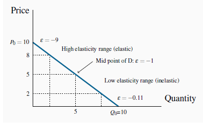
In the high-price region of the demand curve the elasticity takes on a high value. At the midpoint of a linear demand curve the elasticity takes on a value of one, and at lower prices the elasticity value continues to fall.
Using this rule, consider now the value of  when price
drops from $10.00 to $8.00. The change in price is $2.00 and the average price is therefore $9.00 [= ($10.00 + $8.00)/2]. On the quantity side, demand goes from zero to 2 units (measured in
thousands of cubic feet), and the average quantity demanded is therefore (0 + 2)/2 = 1. Putting these numbers into the formula yields:
when price
drops from $10.00 to $8.00. The change in price is $2.00 and the average price is therefore $9.00 [= ($10.00 + $8.00)/2]. On the quantity side, demand goes from zero to 2 units (measured in
thousands of cubic feet), and the average quantity demanded is therefore (0 + 2)/2 = 1. Putting these numbers into the formula yields:
Note that the price has declined in this instance and thus DP is negative. Continuing down the table in this fashion yields the full set of elasticity values in the third column.
The demand elasticity is said to be high if it is a large negative number; the large number denotes a high degree of sensitivity. Conversely, the elasticity is low if it is a small negative number. High and low refer to the size of the number, ignoring the negative sign. The term arc elasticity is also used to define what we have just measured, indicating that it defines consumer responsiveness over a segment or arc of the demand curve.
The arc elasticity of demand defines consumer
responsiveness over a segment or arc of the demand curve.
It is helpful to analyze this numerical example by means of the corresponding demand curve that is plotted in Figure 4.1. It is a straight-line demand curve; but, despite this, the elasticity is not constant. At high prices the elasticity is high; at low prices it is low. The intuition behind this pattern is as follows: When the price is high, a given price change represents a small percentage change, whereas the resulting percentage quantity change will be large. The large percentage quantity change results from the fact that, at the high price, the quantity consumed is small, and, therefore, a small number goes into the denominator of the percentage quantity change. In contrast, when we move to a lower price range on the demand function, a given absolute price change is large in percentage terms, and the resulting quantity change is smaller in percentage terms.
- 8563 reads
