Using information on the slope of the demand curve

Available under Creative Commons-NonCommercial-ShareAlike 4.0 International License.

The elasticity formula, Equation 4.1 part (c), indicates that we could also compute the elasticity values using information on the slope of the demand curve, $\Delta Q/\Delta P$ , multiplied by the appropriate price-quantity ratio. (Note that, even though we put price on the vertical axis, the slope of the demand curve is $\Delta Q/\Delta P$ , as explained in The classical marketplace – demand and supply; $\Delta P/\Delta Q$ is the inverse of this slope, or the slope of the inverse demand function.) Consider the price change from $10.00 to $8.00 again. Columns 1 and 2 indicate that $\Delta Q/\Delta P$ = -2/$2.00, or by simply looking at the equation for the demand curve we can see that its slope is -1. Choosing again the midpoint values for price and quantity yields P/Q = $9.00/1. Therefore the elasticity is

$\varepsilon d = (\Delta Q/\Delta P) = -1_(9.00/1.00) =-9$

Knowing the slope of the demand curve can be very useful in establishing elasticity values when the demand curve is not linear, or when price changes are miniscule, or when the curve intersects the axes. Let us consider each of these cases in turn.

A non-linear demand curve is illustrated in Figure 4.3. If price increases from $P_{}0$ to $P_{}1$ , then over that range we can approximate the slope by the ratio ( $P_{}1$ - $P_{}0$ )=( $Q_{1}$ - $Q_{}0$ ). This is, essentially, an average slope over the range in question that can be used in the formula, in conjunction with an average price and quantity of these values.

Figure 4.3 Non-linear demand curves

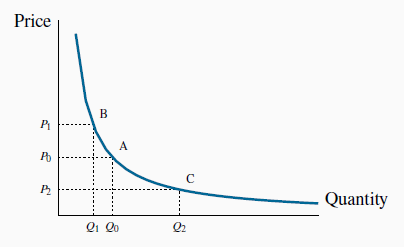
When the demand curve is non-linear the slope changes with the price. Hence, equal price changes do not lead to equal quantity changes: The quantity change associated with a change in price from $P_{}0$ to $P_{}1$ is smaller than the change in quantity associated with the same change in price from $P_{}0$ to $P_{}2$ .

When a price change is infinitesimally small the resulting estimate is called a point elasticity of demand. This differs slightly from the elasticity in column 3 of Table 4.1. In that case, we computed the elasticity along different segments or arcs of the demand function. In Table 4.1, the point elasticity at the point P = $8.00 is

$\varepsilon d = (\Delta Q/\Delta P) = -1X(8.00/2.00) =-4$

The first term in this expression states that quantity changes by 1 unit for each $1 change in price, and the second term states that the elasticity is being evaluated at the price-quantity combination P = $8 and Q = 2. The value of the point elasticity at each price value listed in Table 4.1 is given in column 4. The arc elasticity values in column 3 span a price range, whereas the point elasticities correspond exactly to each price value.

$\mid$ The point elasticity of demand is the elasticity computed at a particular point on the demand curve.

This point elasticity formula can also be applied to the non-linear demand curve in Figure 4.3. If we wished to compute this elasticity exactly at $P_{}2$ , we could draw a tangent to the function at C and evaluate its slope. This slope could then be used in conjunction with the price-quantity combination ( $P_{}2$ , $Q_{2}$ ) to evaluate $\varepsilon d$ at that point.

Next, note that when a demand curve intersects the horizontal axis the elasticity value is zero, regardless of the slope. Using Figure 4.1, we can see that this is because the price in the P/Q component of the elasticity formula equals zero at the intersection point $Q_{}0$ . Hence P/Q = 0 and the elasticity is therefore zero. Likewise, when approaching an intersection with the vertical axis, defined by the point $P_{}0$ in Figure 4.1, the denominator in the P/Q component becomes very small, making the P/Q ratio very large. As we get ever closer to the vertical axis, this ratio becomes correspondingly larger, and therefore we say that the elasticity approaches infinity.

3431 reads

You are here

Using information on the slope of the demand curve