


Despite enormous public interest in taxation and its impact on the economy, it is one of the least understood areas of public policy. In this section we will show how an understanding of two fundamental tools of analysis—elasticities and economic surplus—provides powerful insights into the field of taxation.
We begin with the simplest of cases, the federal government’s goods and services tax (GST) or the provincial governments’ sales taxes (PST). These taxes combined vary by province, but we
suppose that a typical rate is 13 percent. Note that this is a percentage, or ad valorem, tax, not a specific tax of so many dollars per unit traded. Figure 5.3 illustrates the supply and demand curves for some commodity.
In the absence of taxes, the equilibrium  is defined by the
combination (
is defined by the
combination ( ,
,  ).
).
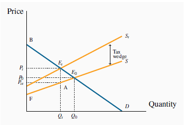
The tax shifts S to  and reduces the quantity traded
from
and reduces the quantity traded
from  to
to  . At
. At  the demand value placed on an additional unit exceeds the supply valuation by EtA. Since the tax keeps output at this lower
level, the economy cannot take advantage of the additional potential surplus between
the demand value placed on an additional unit exceeds the supply valuation by EtA. Since the tax keeps output at this lower
level, the economy cannot take advantage of the additional potential surplus between  and
and  . Excess burden = deadweight loss =
  .
.
A 13-percent tax is now imposed, and the new supply curve  lies 13 percent above the no-tax supply S. A tax wedge is therefore imposed between the price the consumer must pay and the price that the supplier receives. The new equilibrium
is
lies 13 percent above the no-tax supply S. A tax wedge is therefore imposed between the price the consumer must pay and the price that the supplier receives. The new equilibrium
is  , and the new market price is at
  . The price received by the supplier is lower than that paid by the buyer by the
amount of the tax wedge. The post-tax supply price is denoted by
. The price received by the supplier is lower than that paid by the buyer by the
amount of the tax wedge. The post-tax supply price is denoted by  .
.
There are two burdens associated with this tax. The first is the revenue burden, the amount of tax revenue paid by the market participants and received by the government. On each of
the  units sold, the government receives the amount
  . Therefore, tax revenue is the amount
  . As illustrated in Measures of response: elasticities, the degree to which the market price
  rises above the no-tax price
  depends on the supply and demand elasticities.
 A tax wedge is the difference between the consumer
and producer prices.
A tax wedge is the difference between the consumer
and producer prices.
 The revenue burden is the amount of tax revenue
raised by a tax.
The revenue burden is the amount of tax revenue
raised by a tax.
The second burden of the tax is called the excess burden. The concepts of consumer and producer surpluses help us comprehend this. The effect of the tax has been to reduce consumer surplus by
 . This is the reduction in the pre-tax surplus given
by the triangle
. This is the reduction in the pre-tax surplus given
by the triangle  . By the same reasoning, supplier surplus is
reduced by the amount
. By the same reasoning, supplier surplus is
reduced by the amount  ; prior to the tax it was
 . Consumers and suppliers have therefore seen a reduction in
their well-being that is measured by these dollar amounts. Nonetheless, the government has additional revenues amounting to , and this tax imposition therefore represents a transfer from the consumers and suppliers
in the marketplace to the government. Ultimately, the citizens should benefit from this revenue when it is used by the government, and it is therefore not considered to be a net loss of
surplus.
. Consumers and suppliers have therefore seen a reduction in
their well-being that is measured by these dollar amounts. Nonetheless, the government has additional revenues amounting to , and this tax imposition therefore represents a transfer from the consumers and suppliers
in the marketplace to the government. Ultimately, the citizens should benefit from this revenue when it is used by the government, and it is therefore not considered to be a net loss of
surplus.
However, there remains a part of the surplus loss that is not transferred, the triangular area  . This component is called the excess burden, for the reason that it represents the component of the economic surplus that is not
transferred to the government in the form of tax revenue. It is also called the deadweight loss, DWL.
. This component is called the excess burden, for the reason that it represents the component of the economic surplus that is not
transferred to the government in the form of tax revenue. It is also called the deadweight loss, DWL.
 The excess burden, or deadweight loss, of a tax is
the component of consumer and producer surpluses forming a net loss to the whole economy.
The excess burden, or deadweight loss, of a tax is
the component of consumer and producer surpluses forming a net loss to the whole economy.
The intuition behind this concept is not difficult. At the output  , the value placed by consumers on the last unit supplied is
  , while the production cost of that last unit is
  . But the potential surplus
  associated with producing an additional unit cannot be realized, because the tax dictates that the production equilibrium is
at
associated with producing an additional unit cannot be realized, because the tax dictates that the production equilibrium is
at  rather than any higher output. Thus, if output could be
increased from
rather than any higher output. Thus, if output could be
increased from  to
to  , a surplus of value over cost would be realized on every additional unit equal to the
vertical distance between the demand and supply functions D and S. Therefore, the loss associated with the tax is the area .
, a surplus of value over cost would be realized on every additional unit equal to the
vertical distance between the demand and supply functions D and S. Therefore, the loss associated with the tax is the area .
In public policy debates, this excess burden is rarely discussed. The reason is that notions of consumer and producer surpluses are not well understood by non-economists, despite the fact that the value of lost surpluses can be very large. Numerous studies have attempted to estimate the excess burden associated with raising an additional dollar from the tax system. They rarely find that the excess burden is less than 25 percent. This is a sobering finding. It tells us that if the government wished to implement a new program by raising additional tax revenue, the benefits of the new program should be 25 percent greater than the amount expended on it!
The impact of taxes and other influences that result in an inefficient use of the economy’s resources are frequently called distortions. The examples we have developed in this chapter indicate that distortions can describe either an inefficient output being produced, as in the taxation example, or an inefficient allocation of a given output, as in the case of apartments being allocated by lottery.
 A distortion in resource allocation means that
production is not at an efficient output, or a given output is not efficiently allocated.
A distortion in resource allocation means that
production is not at an efficient output, or a given output is not efficiently allocated.
- 2968 reads
