Intuitive Way of Solving Op-Amp Circuits

Available under Creative Commons-ShareAlike 4.0 International License.

When we meet op-amp design specifications, we can simplify our circuit calculations greatly, so much so that we don't need the op-amp's circuit model to determine the transfer function. Here is our inverting amplifier.

Figure 3.45 op-amp

Figure 3.46 op-amp 2

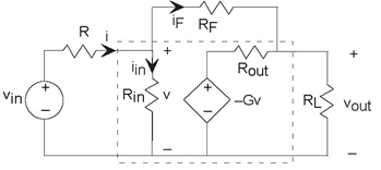
When we take advantage of the op-amp's characteristics large input impedance, large gain, and small output impedance we note the two following important facts.

The current i_in must be very small. The voltage produced by the dependent source is 10⁵ times the voltage v. Thus, the voltage v must be small, which means that $i_{in}=\frac{v}{R_{in}}$ in must be tiny. For example, if the output is about 1 V, the voltage v = 10⁻⁵V, making the current i_in = 10⁻¹¹ A. Consequently, we can ignore i_in in our calculations and assume it to be zero.
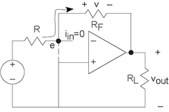
Because of this assumption essentially no current flow through R_in the voltage v must also be essentially zero. This means that in op-amp circuits, the voltage across the op-amp's input is basically zero.

Armed with these approximations, let's return to our original circuit as shown in Figure 3.46. The node voltage e is essentially zero, meaning that it is essentially tied to the reference node. Thus, the current through the resistor R equals $\frac{v_{in}}{R}$ . Furthermore, the feedback resistor appears in parallel with the load resistor. Because the current going into the op-amp is zero, all of the current flowing through R flows through the feedback resistor (iF = i)! The voltage across the feedback resistor v equals $\frac{v_{in}R_F}{R}$ . Because the left end of the feedback resistor is essentially attached to the reference node, the voltage across it equals the negative of that across the output resistor: $v_{out}=-v=-\left ( \frac{v_{in}R_F}{R} \right )$ . Using this approach makes analyzing new op-amp circuits much easier. When using this technique, check to make sure the results you obtain are consistent with the assumptions of essentially zero current entering the op-amp and nearly zero voltage across the op-amp's inputs.

Example 3.8

Figure 3.47 Two Source Circuit

Two-source, single-output op-amp circuit example.

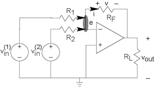
Let's try this analysis technique on a simple extension of the inverting amplifier confguration shown in Figure 3.47 (Two Source Circuit). If either of the source-resistor combinations were not present, the inverting amplifier remains, and we know that transfer function. By superposition, we know that the input-output relation is
$v_{out}=-\left ( \frac{R_F}{R_1}v_{in} \right )-\frac{R_F}{R_2}v_{in}^{\left ( 2 \right )}$
When we start from scratch, the node joining the three resistors is at the same potential as the reference, $e\simeq 0$ , and the sum of currents flowing into that node is zero. Thus, the current i flowing in the resistor RF equals $\frac{v_{in}}{R_1}+\frac{v_{in}}{R_2}$ . Because the feedback resistor is essentially in parallel with the load resistor, the voltages must satisfy v = −v_out. In this way, we obtain the input-output relation given above.

What utility does this circuit have? Can the basic notion of the circuit be extended without bound?

4771 reads

You are here

Intuitive Way of Solving Op-Amp Circuits