Optimization

Available under Creative Commons-NonCommercial-ShareAlike 4.0 International License.

We are now in a position to examine how the consumer optimizes—how he gets to the highest level of satisfaction possible. The constraint on his behaviour is the affordable set defined in Figure 6.6, the budget line.

Figure 6.9 displays several of Neal’s indifference curves in conjunction with his budget constraint. We propose that he maximizes his utility, or satisfaction, at the point E, on the indifference curve denoted by U_3 . While points such as F and G are also on the boundary of the affordable set, they do not yield as much satisfaction as E, because E lies on a higher indifference curve. The highest possible level of satisfaction is attained, therefore, when the budget line touches an indifference curve at just a single point—that is, where the constraint is tangent to the indifference curve. E is such a point.

Figure 6.9 The consumer optimum

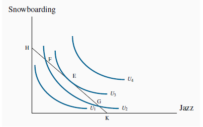
The budget constraint constrains the individual to points on or below HK. The highest level of satisfaction attainable is U_3 , where the budget constraint just touches, or is just tangent to, it. At this optimum the slope of the budget constraint $( - P_{j}/P_{s})$ equals the MRS.

This tangency between the budget constraint and an indifference curve requires that the slopes of each be the same at the point of tangency. We have already established that the slope of the budget constraint is the negative of the price ratio $( - P_{x}/P_{y})$ . The slope of the indifference curve is the marginal rate of substitution MRS. It follows, therefore, that the consumer optimizes where the marginal rate of substitution equals the slope of the price line.

$MRS = \frac{P_{j}}{P_{s}}.$

(6.6)

$\mid$ A consumer optimum occurs where the chosen consumption bundle is a point such that the price ratio equals the marginal rate of substitution.

Notice the resemblance between this condition and the one derived in the first section as Equation 6.2. There we argued that equilibrium requires the marginal utility per dollar expended to be equal for each good:

$\frac{MU_{j}}{P_{j}}=\frac{MU_{s}}{P_{s}}\Rightarrow \frac{MU_{j}}{MU_{s}}=\frac{P_{j}}{P_{s}}$

(6.7)

In fact, with a little mathematics it can be shown that the MRS is indeed the same as the (negative of the) ratio of the marginal utilities: MRS $=MU_{j}=MU_s$ . Therefore the two conditions are in essence the same! However, it was not necessary to assume that an individual can actually measure his utility in obtaining the result that the MRS should equal the price ratio in equilibrium. The concept of ordinal utility is sufficient.

1032 reads

You are here

Optimization