Infinitesimals

Available under Creative Commons-ShareAlike 4.0 International License.

Actually mathematicians have invented many different logical systems for working with infinity, and in most of them infinity does come in different sizes and flavors. Newton, as well as the German mathematician Leibniz who invented calculus independently, 1 had a strong intuitive idea that calculus was really about numbers that were infinitely small: infinitesimals, the opposite of infinities. For instance, consider the number 1.1^2=1.21 . That 2 in the first decimal place is the same 2 that appears in the expression for the derivative of t^2 .

(1.1, 1.21). media/image2.png

Figure 2.2

A close-up view of the function

, showing the line that connects the points (1, 1) and

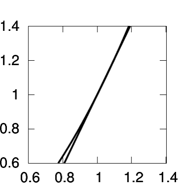
Figure 2.2shows the idea visually. The line connecting the points (1, 1) and (1.1, 1.21) is almost indistinguishable from the tangent line on this scale. Its slope is (1.21 1)/(1.1 1) = 2.1, which is very close to the tangent line's slope of 2. It was a good approximation because the points were close together, separated by only 0.1 on the axis.

If we needed a better approximation, we could try calculating 1.01^2=1.0201 . The slope of the line connecting the points (1, 1) and (1.01, 1.0201) is 2.01, which is even closer to the slope of the tangent line.

Figure 2.3 A geometrical interpretation of the derivative of

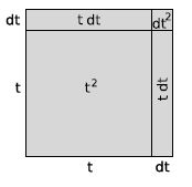
Another method of visualizing the idea is that we can interpret x=t^2 as the area of a square with sides of length , as suggested in Figure 2.3. We increase by an infinitesimally small number . The is Leibniz's notation for a very small difference, and is to be read as a single symbol, "dee-tee," not as a number multiplied by a number . The idea is that is smaller than any ordinary number you could imagine, but it's not zero. The area of the square is increased by dx=2tdt+dt^2 , which is analogous to the finite numbers 0.21 and 0.0201 we calculated earlier. Where before we divided by a finite change in such as 0.1 or 0.01, now we divide by , producing

$\begin{align*} \frac{dx}{dt} &= \frac{2tdt+dt^2}{dt}\\ &= 2t+dt \end{align*}$

for the derivative. On a graph like Figure 2.2, dx/dt is the slope of the tangent line: the change in divided by the changed in .

But adding an infinitesimal number onto doesn't really change it by any amount that's even theoretically measurable in the real world, so the answer is really . Evaluating it at t=1 gives the exact result, 2, that the earlier approximate results, 2.1 and 2.01, were getting closer and closer to.

Example

To show the power of infinitesimals and the Leibniz notation, let’s prove that the derivative of t^3 is 3t^2 : $\begin{align*} \frac{dx}{dt} &=\frac{(t+dt)^3-t^3}{dt} \\ &=\frac{3t^2dt+3tdt^2+dt^3}{dt} \\ &= 3t^2+... \end{align*}$

where the dots indicate infinitesimal terms that we can neglect.

This result required significant sweat and ingenuity when proved on Derivatives of polynomials by the methods of Rates of Change, and not only that but the old method would have required a completely different method of proof for a function that wasn't a polynomial, whereas the new one can be applied more generally, as we'll see presently in Example;Example;Example and Example.

It's easy to get the mistaken impression that infinitesimals exist in some remote fairyland where we can never touch them. This may be true in the same artsy-fartsy sense that we can never truly understand $\sqrt{2}$ , because its decimal expansion goes on forever, and we therefore can never compute it exactly. But in practical work, that doesn't stop us from working with $\sqrt{2}$ . We just approximate it as, e.g., 1.41. Infinitesimals are no more or less mysterious than irrational numbers, and in particular we can represent them concretely on a computer. If you go to $\texttt{lightandmatter.com/calc/inf}$ , you'll find a web-based calculator called Inf, which can handle infinite and infinitesimal numbers. It has a built-in symbol, d, which represents an infinitesimally small number such as the dx's and dt's we've been handling symbolically.

Let's use Inf to verify that the derivative of t^3 , evaluated at t=1 , is equal to 3, as found by plugging in to the result of Example. The : symbol is the prompt that shows you Inf is ready to accept your typed input.

: ((1+d)^3-1)/d
3+3d+d^2

As claimed, the result is 3, or close enough to 3 that the infinitesimal error doesn't matter in real life. It might look like Inf did this example by using algebra to simplify the expression, but in fact Inf doesn't know anything about algebra. One way to see this is to use Inf to compare d with various real numbers:

: d<1
true
: d<0.01
true
: d<0.0000001
true
: d<0
false

If d were just a variable being treated according to the axioms of algebra, there would be no way to tell how it compared with other numbers without having some special information. Inf doesn't know algebra, but it does know that d is a positive number that is less than any positive real number that can be represented using decimals or scientific notation.

Example

In Example, we made a rough numerical check to see if the differentiation rule $t^k\rightarrow kt^{k-1}$ , which was proved on Derivatives of polynomials for k=1,2,3,... , was also valid for k=-1 , i.e., for the function x=1/t . Let’s look for an actual proof. To find a natural method of attack, let’s first redo the numerical check in a slightly more suggestive form. Again approximating the derivating at t=3 , we have

$\frac{dx}{dt}\approx \left ( \frac{1}{3.01}-\frac{1}{3} \right )\left ( \frac{1}{0.01} \right )$

Let’s apply the grade-school technique for subtracting fractions, in which we first get them over the same denominator:

$\frac{1}{3}-\frac{1}{3.01}=\frac{3-3.01}{3\times 3.01}$

The result is

$\begin{align*} \frac{dx}{dt}&\approx \left ( \frac{1}{3.01}-\frac{1}{3} \right )\left ( \frac{1}{0.01} \right ) \\ &= -\frac{1}{3\times 3.01} \end{align*}$

Replacing 3 with and 0.01 with , this becomes $\begin{align*} \frac{dx}{dt} &=-\frac{1}{t(t+dt)} \\ &= -t^{-2}+... \end{align*}$

Example

The derivative of $x-\textrm{sin }t$ , with in units of radians, is
$\frac{dx}{dt}=\frac{\textrm{sin }(t+dt)-\textrm{sin }t}{dt}$
and with the trig identity $\textrm{sin}(\alpha +\beta )=\textrm{sin }\alpha \textrm{ cos }\beta +\textrm{ cos }\alpha \textrm{ sin }\beta$ , this becomes
$=\frac{\textrm{sin } t \textrm{ cos } dt + \textrm{ cos } t \textrm{ sin } dt - \textrm{ sin } t}{dt}$

Applying the small-angle approximations $\textrm{sin } u\approx u$ and $\textrm{cos } u\approx 1$ we have
$\begin{align*} \frac{dx}{dt} &=\frac{\textrm{cos }t dt}{dt}+\cdots \\ &= \textrm{cos } t+\cdots \end{align*}$
where “. . . ” represents the error caused by the small-angle approximations.
This is essentially all there is to the computation of the derivative, except for the remaining technical point that we haven’t proved that the small-angle approximations are good enough. In Example, when we calculated the derivative of t^3 , the resulting expression for the quotient dx= dt came out in a form in which we could inspect the “. . . ” terms and verify before discarding them that they were infinitesimal. The issue is less trivial in the present example. This point is addressed more rigorously on Details of the proof of the derivative of the sine function

Figure 2.4 Graphs of

$\textrm{sin }t$ , and its derivative $\textrm{cos }t$ .

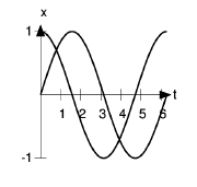
Figure 2.4 shows the graphs of the function and its derivative. Note how the two graphs correspond. At t=0 , the slope of sin t is at its largest, and is positive; this is where the derivative, cos t, attains its maximum positive value of 1. At $t=\pi/2$ , $\textrm{sin }t$ has reached a maximum, and has a slope of zero; $\textrm{cos }t$ is zero here. At $t=\pi$ , in the middle of the graph, sin t has its maximum negative slope, and cos t is at its most negative extreme of -1.

Physically, $\textrm{sin }t$ could represent the position of a pendulum as it moved back and forth from left to right, and cos t would then be the pendulum’s velocity.

Example

What about the derivative of the cosine? The cosine and the sine are really the same function, shifted to the left or right by $\pi/2$ . If the derivative of the sine is the same as itself, but shifted to the left by $\pi/2$ , then the derivative of the cosine must be a cosine shifted to the left by $\pi/2$ :
$\begin{align*} \frac{d \textrm{ cos }t}{dt} &=\textrm{cos }(t+\pi /2) \\ &= -\textrm{sin }t \end{align*}$

The next example will require a little trickery. By the end of this chapter you'll learn general techniques for cranking out any derivative cookbook-style, without having to come up with any tricks.

Example

Figure 2.5 The function

x=1/(1-t)

Find the derivative of 1/(1-t) , evaluated at t=0 .
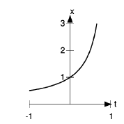
The graph shows what the function looks like. It blows up to infinity at t=1 , but it’s well behaved at t=0 , where it has a positive slope.
For insight, let’s calculate some points on the curve. The point at which we’re differentiating is (0, 1). If we put in a small, positive value of , we can observe how much the result increases relative to 1, and this will give us an approximation to the derivative. For example, we find that at = 0.001, the function has the value 1.001001001001, and so the derivative is approximately (1.0011)/(.001-0), or about 1. We can therefore conjecture that the derivative is exactly 1, but that’s not the same as proving it.

But let’s take another look at that number 1.001001001001. It’s clearly a repeating decimal. In other words, it appears that
$\frac{1}{1-1/1000}=1+\frac{1}{1000}+\left ( \frac{1}{1000} \right )^2+...$
and we can easily verify this by multiplying both sides of the equation by 1-1/1000 and collecting like powers. This is a special case of the geometric series
$\frac{1}{1-t}=1+t+t^2+...$ which can be derived 2 by doing synthetic division (the equivalent of long division for polynomials), or simply verified, after forming the conjecture based on the numerical example above, by multiplying both sides by 1-t.
As we’ll see in Safe use of infinitesimals, and have been implicitly assuming so far, infinitesimals obey all the same elementary laws of algebra as the real numbers, so the above derivation also holds for an infinitesimal value of . We can verify the result using Inf:

: 1/(1-d)
1+d+d^2+d^3+d^4

Notice, however, that the series is truncated after the first five terms. This is similar to the truncation that happens when you ask your calculator to find $\sqrt{2}$ as a decimal.
The result for the derivative is
$\begin{align*} \frac{dx}{dt} &=\frac{(1+dt+dt^2+...)-1}{1+dt-1} \\ &= 1+... \end{align*}$

瀏覽次數：3641

您在這裡

Infinitesimals

Example

Example

Example