Applications Averages

Available under Creative Commons-ShareAlike 4.0 International License.

In the story of Gauss’s problem of adding up the numbers from 1 to100, one interpretation of the result, 5,050, is that the average of all the numbers from 1 to 100 is 50.5. This is the ordinary definition of an average: add up all the things you have, and divide by the number of things. (The result in this example makes sense, because half the numbers are from 1 to 50, and half are from 51 to 100, so the average is half-way between 50 and 51.)

Similarly, a definite integral can also be thought of as a kind of aver- age. In general, if is a function of , then the average, or mean, value of on the interval from x=a to can be defined as $\bar{y}=\frac{1}{b-a}\int_{b}^{a}y \textrm{{ }}dx$
In the continuous case, dividing by b − a accomplishes the same thing as dividing by the number of things in the discrete case.

Example

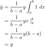
Show that the definition of the average makes sense in the case where the function is a constant.If is a constant, then we can take it outside of the integral, so $\begin{align*} \bar{y} &=\frac{1}{b-a}y\int_{a}^{b}1\textrm{{ }}dx \\ &=\frac{1}{b-a}y x \mid _{a}^{b} \\ &=\frac{1}{b-a}y(b-a) \\ &= y \end{align*}$

Example

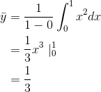
Find the average value of the function y=x^2 for values of ranging from 0 to 1.

$\begin{align*} \bar{y} &=\frac{1}{1-0}\int_{0}^{1}x^2dx \\ &= \frac{1}{3}x^3\mid ^{1}_{0}\\ &= \frac{1}{3} \end{align*}$

The mean value theorem

If the continuous function y(x) has the average value $\bar{y}$ on the interval from x=a to , then attains its average value at least once in that interval, i.e., there exists $\xi$ with $a<\xi <b$ such that $y(\xi )=\bar{y}$ .