Polar coordinates

Available under Creative Commons-ShareAlike 4.0 International License.

Figure 9.2 b/ Rene Descartes (1596-1650)

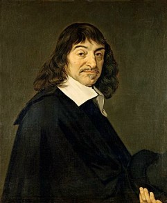
Philosopher and mathematician Ren´e Descartes originated the idea of describing plane geometry using (x, y) coordinates measured from a pair of perpendicular coordinate axes. These rectangular coordinates are known as Cartesian co- ordinates, in his honor.

As a logical extension of Descartes’ idea, one can find different ways of defining coordinates on the plane, such as the polar coordinates in figure c. In polar coordinates, the differential of area, figure d can be written as da= RdRdφ. The idea is that since dRand dφare infinitesimally small, the shaded area in the figure is very nearly a rectangle, measuring dRis one dimension and Rdφin the other. (The latter follows from the definition of radian measure.)

Figure 9.3 c / Polar coordinates.

Figure 9.4 d / The differential of area in polar coordinates

Figure 9.5

Example 98

A disk has mass Mand radius b. Find its moment of inertia for rotation about the axis passing perpendicularly through its center.

$\begin{align*} I&=\int R^{2}dM \\&=\int R^{2}\frac{dM}{da}da \\&=\int R^{2}\frac{M}{\pi b^{2}}da \\&=\frac{M}{\pi b^{2}}\int_{R=0}^{b}\int_{\o =0}^{2\pi }R^{2}\cdot Rd\o dR \\&=\frac{M}{\pi b^{2}}\int_{R=0}^{b}R^{3}\int_{\o =0}^{2\pi }\cdot R\o dR \\&=\frac{2M}{\ b^{2}}\int_{R=0}^{b}R^{3} dR \\&=\frac{Mb^{4}}{2} \end{align*}$

Figure 9.6 e / The function e−x , example 99.

Example 99

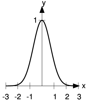
In statistics, the standard “bell curve” (also known as the normal distribution or Gaussian) is shaped like $e^{-x}^{2}$ . An area under this curve is proportional to the probability that xlies within a certain range. To fix the constant ofproportionality, we need to evaluate

$I=\int_{-\infty }^{\infty }e^{-x}^{2}dx,$

which corresponds to a probability of

1. As discussed, the corresponding indefinite Integrals that can’t be done in closed form. The definite integral from −∞ to +∞, however, can be evaluated by the following devious trick due to Poisson. We first write $I^{2}$ as a product of two copies of the integral.

$I^{2}=(\int_{-\infty }^{\infty }e^{-x}^{2}dx)(\int_{-\infty }^{\infty }e^{-x}^{2}dx)$

Since the variable of integration xis a “dummy” variable, we can choose it to be any letter of the alphabet. Let’s change the second one to y:

$I^{2}=(\int_{-\infty }^{\infty }e^{-x}^{2}dx)(\int_{-\infty }^{\infty }e^{-x}^{2}dy)$

This is in principle a pointless and trivial change, but it suggests visualizing the right-hand side in the Cartesian plane, and considering it as the integral of a single function that depends on both x and y:

$I^{2}=\int_{-\infty }^{\infty }\int_{-\infty }^{\infty }(e^{-y}^{2}e^{-x}^{2})dxdy$
Switching to polar coordinates, we have