


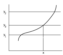
Another way of thinking about continuous functions is given by the intermediate value theorem. Intuitively, it says that if you are moving continuously along a road, and you get from
point A to point B, then you must also visit every other point along the road; only by teleporting (by moving discontinuously) could you avoid doing so. More formally, the theorem states that
if  is a continuous real-valued function on the real interval from a to
 , and if
  takes on
values
takes on
values  and
and  at certain points within this interval, then for any
  between
  and
and
 , there is some real
  in the interval for which
  .
.

The intermediate value theorem seems so intuitively appealing that if we want to set out to prove it, we may feel as though we’re being asked to prove a proposition such as, “a number greater
than 10 exists.” If a friend wanted to bet you a six-pack that you couldn’t prove this with complete mathematical rigor, you would have to get your friend to spell out very explicitly what she
thought were the facts about integers that you were allowed to start with as initial assumptions. Are you allowed to assume that 1 exists? Will she grant you that if a number n exists, so does
 ? The intermediate value theorem is similar. It’s stated as a
theorem about certain types of functions, but its truth isn’t so much a matter of the properties of functions as the properties of the underlying number system. For the reader with a interest
in pure mathematics, I’ve discussed this in more detail in The intermediate value theorem and given an abbreviated proof. (Most introductory calculus texts do not prove it at all.)
? The intermediate value theorem is similar. It’s stated as a
theorem about certain types of functions, but its truth isn’t so much a matter of the properties of functions as the properties of the underlying number system. For the reader with a interest
in pure mathematics, I’ve discussed this in more detail in The intermediate value theorem and given an abbreviated proof. (Most introductory calculus texts do not prove it at all.)
Example
Show that there is a solution to the equation  .
.
We expect there to be a solution near  , where the function
 is just a little too big. On the other hand,
 is much too small. Since
  has values above and below 1000 on the interval from 2 to 3, and
  is continuous, the intermediate
value theorem proves that a solution exists between 2 and 3. If we wanted to find a better numerical approximation to the solution, we could do it using Newton’s method, which is introduced
in Newton’s method.
is continuous, the intermediate
value theorem proves that a solution exists between 2 and 3. If we wanted to find a better numerical approximation to the solution, we could do it using Newton’s method, which is introduced
in Newton’s method.
Example
Show that there is at least one solution to the equation  , and give bounds on its location.
This is a transcendental equation, and no amount of fiddling with algebra and trig identities will ever give a closed-form solution, i.e., one that can be written down with a finite number of
arithmetic operations to give an exact result. However, we can easily prove that at least one solution exists, by applying the intermediate value theorem to the function  . The cosine function is bounded between −1 and 1, so this
function must be negative for
. The cosine function is bounded between −1 and 1, so this
function must be negative for  and positive for
  . By the intermediate value theorem, there must be a solution in the
interval
. By the intermediate value theorem, there must be a solution in the
interval  . The graph, c, verifies this, and shows that
there is only one solution.
. The graph, c, verifies this, and shows that
there is only one solution.
 constructed in Example.
Example
Prove that every odd-order polynomial  with real coefficients has at
least one real root
with real coefficients has at
least one real root  , i.e., a point at which
  .
.
Example might have given the impression that there was nothing to be learned from the intermediate value theorem that couldn’t be deter- mined by graphing, but this example clearly can’t be solved by graphing, because we’re trying to prove a general result for all polynomials.
To see that the restriction to odd orders is necessary, consider the polynomial  , which has no real roots because
  for any real number
  .
.
To fix our minds on a concrete example for the odd case, consider the polynomial  . For large values of
  , the linear and constant terms will be negligible compared to the
  term, and since
  is positive for large values of
 and negative for large negative ones, it follows that
  is sometimes positive and sometimes negative.
Making this argument more general and rigorous, suppose we had a polynomial of odd order  that always had the same sign for real
  . Then by the transfer principle the
same would hold for any hyperreal value of
. Then by the transfer principle the
same would hold for any hyperreal value of  . Now if
  is infinite then the lower-order
terms are infinitesimal compared to the
is infinite then the lower-order
terms are infinitesimal compared to the  term, and the sign of the result is
determined entirely by the
term, and the sign of the result is
determined entirely by the  term, but
  and
and  have opposite signs, and therefore
  and
and  have opposite signs. This is a contradiction, so we have disproved the assumption that
  always had the same sign for real
  . Since
  is sometimes negative and sometimes
positive, we conclude by the intermediate value theorem that it is zero somewhere.
is sometimes negative and sometimes
positive, we conclude by the intermediate value theorem that it is zero somewhere.
Example
Show that the equation  has infinitely many
solutions.
has infinitely many
solutions.
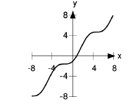
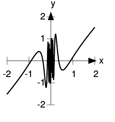
This is another example that can’t be solved by graphing; there is clearly no way to prove, just by looking at a graph like d, that it crosses the x axis infinitely many times. The
graph does, however, help us to gain intuition for what’s going on. As  gets smaller and smaller,
  blows up, and
  oscillates more and more rapidly. The function
  is undefined at 0, but it’s continuous everywhere else, so we can apply the intermediate value theorem to any interval that
doesn’t include 0.
is undefined at 0, but it’s continuous everywhere else, so we can apply the intermediate value theorem to any interval that
doesn’t include 0.
We want to prove that for any positive  , there exists an
  with
with  for which
  has either desired sign. Suppose that this fails for some real
  . Then by the transfer principle the nonexistence of any real
  with the desired property also
implies the nonexistence of any such hyperreal
with the desired property also
implies the nonexistence of any such hyperreal  . But for an infinitesimal
  the sign of
  is determined entirely by the sine
term, since the sine term is finite and the linear term infinitesimal. Clearly
is determined entirely by the sine
term, since the sine term is finite and the linear term infinitesimal. Clearly  can’t have a single sign for all values of
  less than
  , so this is a contradiction, and the
proposition succeeds for any u. It follows from the intermediate value theorem that there are infinitely many solutions to the equation.
, so this is a contradiction, and the
proposition succeeds for any u. It follows from the intermediate value theorem that there are infinitely many solutions to the equation.

- 5422 reads
