


Mathematically, the probability that something will happen can be specified with a number ranging from 0 to 1, with 0 representing impossibility and 1 representing certainty. If you flip a coin, heads and tails both have probabilities of 1/2. The sum of the probabilities of all the possible outcomes has to have probability 1. This is called normalization.
So far we’ve discussed random processes having only two possible outcomes: yes or no, win or lose, on or off. More generally, a random process could have a result that is a number. Some processes yield integers, as when you roll a die and get a result from one to six, but some are not restricted to whole numbers, e.g., the height of a human being, or the amount of time that a uranium-238 atom will exist before undergoing radioactive decay. The key to handling these continuous random variables is the concept of the area under a curve, i.e., an integral.
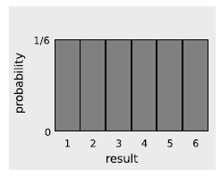
Consider a throw of a die. If the die is “honest,” then we expect all six values to be equally likely. Since all six probabilities must add up to 1, then probability of any particular value coming up must be 1/6. We can summarize this in a graph, f. Areas under the curve can be interpreted as total probabilities. For instance, the area under the curve from 1 to 3 is 1/6+1/6+1/6 = 1/2, so the probability of getting a result from 1 to 3 is 1/2. The function shown on the graph is called the probability distribution.
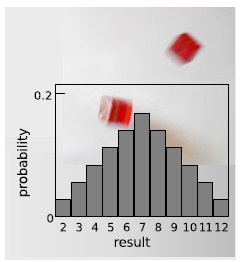
Figure 4.7 shows the probabilities of various results obtained by rolling two dice and adding them together, as in the game of craps. The probabilities are not all the same. There is a small probability of getting a two, for example, be- cause there is only one way to do it, by rolling a one and then another one. The probability of rolling a seven is high because there are six different ways to do it: 1+6, 2+5, etc.
If the number of possible outcomes is large but finite, for example the number of hairs on a dog, the graph would start to look like a smooth curve rather than a ziggurat.
What about probability distributions for random numbers that are not integers? We can no longer make a graph with probability on the y axis, because the probability of getting a given exact number is typically zero. For instance, there is zero probability that a per- son will be exactly 200 cm tall, since there are infinitely many possible results that are close to 200 but not exactly two, for example 199.99999999687687658766. It doesn’t usually make sense, therefore, to talk about the probability of a single numerical result, but it does make sense to talk about the probability of a certain range of results. For instance, the probability that a randomly chosen person will be more than 170 cm and less than 200 cm in height is a perfectly reasonable thing to discuss. We can still summarize the probability in- formation on a graph, and we can still interpret areas under the curve as probabilities.

But the  axis can no longer be a unitless probability scale. In the
example of human height, we want the
axis can no longer be a unitless probability scale. In the
example of human height, we want the  axis to have units of meters, and
we want areas under the curve to be unitless probabilities. The area of a single square on the graph paper is then
axis to have units of meters, and
we want areas under the curve to be unitless probabilities. The area of a single square on the graph paper is then

If the units are to cancel out, then the height of the square must evidently be a quantity with units of inverse centimeters. In other words, the  axis of the graph is to be interpreted as probability per unit height, not probability.
Another way of looking at it is that the  axis on the graph gives a derivative,
  : the infinitesimally small probability that
  will lie in the infinitesimally small range covered by
  .
.
Example
A computer language will typically have a built-in subroutine that produces a fairly random number that is equally likely to take on any value in the range from 0 to 1. If you take the
absolute value of the difference between two such numbers, the probability distribution is of the form  . Find the value of the constant
  that is required by normalization.
Self-Check.
Compare the number of people with heights in the range of 130-135 cm to the number in the range 135-140.
Answers to self-checks for chapter 4

When one random variable is related to another in some mathematical way, the chain rule can be used to relate their probability distributions.
Example
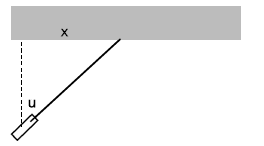
A laser is placed one meter away from a wall, and spun on the ground to give it a random direction, but if the angle 
 shown in Figure 4.10 doesn’t come out in the range from 0 to
  , the laser is spun again until an angle in the desired range is obtained. Find the probability distribution of the distance
 shown in the figure. The derivative
  will be required (see Example).
Since any angle between 0 and  is equally likely, the probability
distribution
is equally likely, the probability
distribution  must be a constant, and normalization tells us
that the constant must be
must be a constant, and normalization tells us
that the constant must be  .
.
The laser is one meter from the wall, so the distance  , measured in
meters, is given by
, measured in
meters, is given by  . For the probability
distribution of
. For the probability
distribution of  , we have
Note that the range of possible values of  theoretically extends
from 0 to infinity. Problem 6.7 deals with this.
theoretically extends
from 0 to infinity. Problem 6.7 deals with this.
If the next Martian you meet asks you, “How tall is an adult hu- man?,” you will probably reply with a statement about the average human height, such as “Oh, about 5 feet 6 inches.” If you
wanted to explain a little more, you could say, “But that’s only an average. Most people are somewhere between 5 feet and 6 feet tall.” Without bothering to draw the relevant bell curve for
your new extraterrestrial acquaintance, you’ve summarized the relevant information by giving an average and a typical range of variation. The average of a probability distribution can be
defined geometrically as the horizontal position at which it could be balanced if it was constructed out of cardboard, i. This is a different way of working with averages than the one we did
earlier. Before, had a graph of  versus
  , we implicitly assumed that all values of
  were equally likely, and we found an average value of
  . In this new method using probability distributions, the variable we’re
averaging is on the
. In this new method using probability distributions, the variable we’re
averaging is on the  axis, and the
  axis tells
us the relative probabilities of the various
axis tells
us the relative probabilities of the various  values.
For a discrete-valued variable with  possible values, the average
would be
possible values, the average
would be
and in the case of a continuous variable, this becomes an integral,
 .
.
Sometimes we don’t just want to know the average value of a certain variable, we also want to have some idea of the amount of variation above and below the average. The most common way of measuring this is the standard deviation, defined by
The idea here is that if there was no variation at all above or below the average, then the quantity  would be zero whenever
  was nonzero, and the standard deviation would be zero. The reason for taking the square root of the whole thing is so that the
result will have the same units as
was nonzero, and the standard deviation would be zero. The reason for taking the square root of the whole thing is so that the
result will have the same units as  .
.
Example
For the situation described in exam- ple 59, find the standard deviation of  .
.
The square of the standard deviation is
 so the standard deviation is

- 3460 reads
