Definite and indefinite integrals

Available under Creative Commons-ShareAlike 4.0 International License.

Because any formula can be differentiated symbolically to find an- other formula, the main motivation for doing derivatives numerically would be if the function to be differentiated wasn’t known in symbolic form. A typical example might be a two-person network computer game, in which player A’s computer needs to figure out player B’s velocity based on knowledge of how her position changes over time. But in most cases, it’s numerical integration that’s interesting, not numerical differentiation.

As a warm-up, let’s see how to do a running sum of a discrete function using Yacas. The following program computes the sum 1+2+...+100 discussed to in Change in discrete steps. Now that we’re writing real computer programs with Yacas, it would be a good idea to enter each program into a file before trying to run it. In fact, some of these examples won’t run properly if you just start up Yacas and type them in one line at a time. If you’re using Adobe Reader to read this book, you can do $\texttt{Tools>Basic>Select}$ , select the program, copy it into a file, and then edit out the line numbers.

Example

n := 1;
sum := 0;
While (n<=100) [
sum := sum+n;
n := n+1;
];
Echo(sum)

The semicolons are to separate one instruction from the next, and they become necessary now that we’re doing real programming. Line 1 of this program defines the variable n, which will take on all the values from 1 to 100. Line 2 says that we haven’t added anything up yet, so our running sum is zero so far. Line 3 says to keep on repeating the instructions inside the square brackets until n goes past 100. Line 4 updates the running sum, and line 5 updates the value of n. If you’ve never done any programming before, a statement like $\texttt{n:=n+1}$ might seem like nonsense — how can a number equal itself plus one? But that’s why we use the := symbol; it says that we’re redefining $\texttt{n}$ , not stating an equation. If $\texttt{n}$ was previously 37, then after this statement is executed, n will be redefined as 38. To run the program on a Linux computer, do this (assuming you saved the pro- gram in a file named $\texttt{sum.yacas}$ ):

yacas -pc sum.yacas
5050

Here the % symbol is the computer’s prompt. The result is 5,050, as expected. 　 One way of stating this result is $\sum _{n=1}^{100}n=5050$
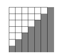
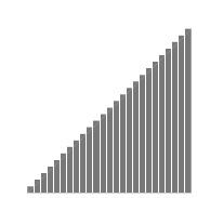
The capital Greek letter $\sum$ , sigma, is used because it makes the “s” sound, and that’s the first sound in the word “sum.” The n=1 below the sigma says the sum starts at 1, and the 100 on top says it ends at 100. The is what’s known as a dummy variable: it has no meaning outside the context of the sum. Figure 4.1 shows the graphical interpretation of the sum: we’re adding up the areas of a series of rectangular strips. (For clarity, the figure only shows the sum going up to 7, rather than 100.)

Figure 4.1 Graphical interpretation of the sum 1+2+...+7

Now how about an integral? Figure 4.2 shows the graphical interpretation of what we’re trying to do: find the area of the shaded triangle. This is an example we know how to do symbolically, so we can do it numerically as well, and check the answers against each other. Symbolically, the area is given by the integral. To integrate the function $\dot{x}(t)=t$ , we know we need some function with a t^2 in it, since we want something whose derivative is , and differentiation reduces the power by one. The derivative of t^2 would be rather than , so what we want is x(t)=t^2/2 . Let’s compute the area of the triangle that stretches along the axis from 0 to 100: x(100)=100^2/2=5000 .

Figure 4.2 Graphical interpretation of the integral of the function

$\dot{x}(t)=t$

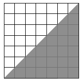
Figure 4.3 shows how to accomplish the same thing numerically. We break up the area into a whole bunch of very skinny rectangles. Ideally, we’d like to make the width of each rectangle be an infinitesimal number , so that we’d be adding up an infinite number of infinitesimal areas. In reality, a computer can’t do that, so we divide up the interval from t=0 to t=100 into rectangles, each with finite width dt=100/H . Instead of making H infinite, we make it the largest number we can without making the computer take too long to add up the areas of the rectangles.

Figure 4.3 Approximating the integral numerically.

Example

tmax := 100;
H := 1000;
dt := tmax/H;
sum := 0;
t := 0;
While (t<=tmax) [
 sum := N(sum+t*dt);
 t := N(t+dt);
];
 Echo(sum);

In Example, we split the interval from t=0 to 100 into H=1000 small intervals, each with width dt=0.1 . The result is 5,005, which agrees with the symbolic result to three digits of precision. Changing to 10,000 gives 5, 000.5, which is one more digit. Clearly as we make the number of rectangles greater and greater, we're converging to the correct result of 5,000.

In the Leibniz notation, the thing we've just calculated, by two different techniques, is written like this:

$\int_{0}^{100}t\textrm{d}t=5,000$ It looks a lot like the $\sum$ notation, with the $\sum$ replaces by a flattened out letter “S.” The is a dummy variable. What I’ve been casually referring to as an integral is re- ally two different but closely related things, known as the definite integral and the indefinite integral.

Definition of the indefinite integral

If $\dot{x}$ is a function, then a function is an indefinite integral of $\dot{x}$ if, as implied by the notation, $dx/dt=\dot{x}$ .

Interpretation: Doing an indefinite integral means doing the opposite of differentiation. All the possible indefinite integrals are the same function except for an additive constant.

Example

Find the indefinite integral of the function $\dot{x}(t)=t$ .

Any function of the form

x(t)=t^2/2+c

where is a constant, is an indefinite integral of this function, since its derivative is .

Definition of the definite integral

If $\dot{x}$ is a function, then the definite integral of $\dot{x}$ from a to b is defined as

$\int _{a}^{b}\dot{x}(t)dt \\=\lim_{H\rightarrow \infty}\sum_{i=0}^{H}\dot{x}(a+i\Delta t)\Delta t$

where $\Delta t=(b-a)/H$

Interpretation: What we’re calculating is the area under the graph of $\dot{x}$ , from to . (If the graph dips below the axis, we interpret the area between it and the axis as a negative area.) The thing inside the limit is a calculation like the one done in Example, but generalized to $a\neq 0$ . If was infinite, then $\Delta t$ would be an infinitesimal number .

2908 reads

You are here

Definite and indefinite integrals

Example

Example

Definition of the indefinite integral

Example

Definition of the definite integral