


Did you notice that I sneaked something past you in the example of water filling up a reservoir? The  and
and  functions I've been using as examples have all been functions defined on the integers, so they represent change that happens in
discrete steps, but the flow of water into a reservoir is smooth and continuous. Or is it? Water is made out of molecules, after all. It's just that water molecules are so small that we don't
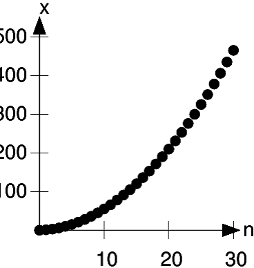
notice them as individuals. Figure 1.7 shows a graph
that is discrete, but almost appears continuous because the scale has been chosen so that the points blend together visually.
functions I've been using as examples have all been functions defined on the integers, so they represent change that happens in
discrete steps, but the flow of water into a reservoir is smooth and continuous. Or is it? Water is made out of molecules, after all. It's just that water molecules are so small that we don't
notice them as individuals. Figure 1.7 shows a graph
that is discrete, but almost appears continuous because the scale has been chosen so that the points blend together visually.
 appears almost continuous.
The physicist Isaac Newton started thinking along these lines in the 1660's, and figured out ways of analyzing  and
and
 functions that were truly continuous. The notation
  is due to him (and he only used it for continuous functions). Because he
was dealing with the continuous flow of change, he called his new set of mathematical techniques the method of fluxions, but nowadays it's known as the calculus.
is due to him (and he only used it for continuous functions). Because he
was dealing with the continuous flow of change, he called his new set of mathematical techniques the method of fluxions, but nowadays it's known as the calculus.
 ,and its tangent line at the point (1,
1=2).
,and its tangent line at the point (1,
1=2).
Newton was a physicist, and he needed to invent the calculus as part of his study of how objects move. If an object is moving in one dimension, we can specify its position with a variable
 , and
, and  will
then be a function of time,
will
then be a function of time,  . The rate of change of its position,
 , is its speed, or velocity. Earlier experiments by Galileo had
established that when a ball rolled down a slope, its position was proportional to
, is its speed, or velocity. Earlier experiments by Galileo had
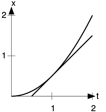
established that when a ball rolled down a slope, its position was proportional to  , so Newton inferred that a graph like Figure 1.8 would be typical for any object moving under the influence of a constant force. (It could be
  , or
, or  , or anything else proportional to
  , depending on the force acting on the object and the object's mass.)
Because the functions are continuous, not discrete, we can no longer define the relationship between  and
and
 by saying
  is a running sum of
  's, or that x_ is the difference between two successive
  's. But we already found a geometrical relationship between the two
functions in the discrete case, and that can serve as our definition for the continuous case:
's. But we already found a geometrical relationship between the two
functions in the discrete case, and that can serve as our definition for the continuous case:  is
the area under the graph of
is
the area under the graph of  , or, if you like,
  is the slope of the graph of
  . For now we'll concentrate on the slope idea.
This definition is still a little vague, because we haven't defined what we mean by the "slope" of a curving graph. For a discrete graph like Figure 1.4, we could define it as the slope of the line drawn between neighboring points. Visually, it's clear that the continuous version of this is something like the line drawn in Figure 1.8. This is referred to as the tangent line.
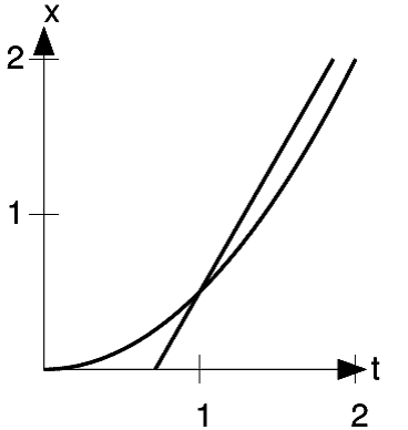
We still need to convert this intuitive idea of a tangent line into a formal definition. In a typical example like figure h, the tangent line can be defined as the line that touches the graph
at a certain point, but, unlike the line in Figure 1.9, doesn't cut across
the graph at that point. 1 By measuring with a ruler on
Figure 1.8, we find that the slope is very close to 1, so evidently  . To prove this, we construct the function representing the line:
 . We want to prove that this line doesn't cross the graph of
 . The difference between the two functions,
  , is the polynomial
  , and this polynomial will be zero for any value of
  where the line touches or crosses the curve. We can use the quadratic
formula to _nd these points, and the result is that there is only one of them, which is
where the line touches or crosses the curve. We can use the quadratic
formula to _nd these points, and the result is that there is only one of them, which is  . Since
  is positive for at least some points to the left and right of
  , and
it only equals zero at
, and
it only equals zero at  , it must never be negative, which means that
the line always lies below the curve, never crossing it.
, it must never be negative, which means that
the line always lies below the curve, never crossing it.
- 瀏覽次數:2790
