


Losses are activities that absorb resources without creating value. Losses can be divided by their frequency of occurrence, their cause and by different types they are. The latter one has been developed by Nakajima1 and it is the well-known Six Big Losses framework. The other ones are interesting in order to rank rightly losses.
According to Johnson et al.2, losses can be chronic or sporadic. The chronic disturbances are usually described as “small, hidden and complicated” while the sporadic ones occur quickly and with large deviations from the normal value. The loss frequency combined with the loss severity gives a measure of the damage and it is useful in order to establish the order in which the losses have to be removed. This classification makes it possible to rank the losses and remove them on the basis of their seriousness or impact on the organization.
Regarding divide losses by their causes, three different ones can be found:
- machine malfunctioning: an equipment or a part of this does not fulfill the demands;
- process: the way the equipment is used during production;
- external: cause of losses that cannot be improved by the maintenance or production team.
The external causes such as shortage of raw materials, lack of personnel or limited demand do not touch the equipment effectiveness. They are of great importance for top management and they should be examined carefully because their reduction can directly increase the revenues and profit. However they are not responsible of the production or maintenance team and so they are not taken into consideration through the OEE metric.
To improve the equipment effectiveness the losses because of external causes have to be taken out and the losses caused by machine malfunctioning and process, changeable by the daily organization, can still be divided into:
- Down time losses: when the machine should run, but it stands still. Most common downtime losses happen when a malfunction arises, an unplanned maintenance task must be done in addition to the big revisions or a set-up/start-up time occurs.
- Speed losses: the equipment is running, but it is not running at its maximum designed speed. Most common speed losses happen when equipment speed decrease but it is not zero. It can depend on a malfunctioning, a small technical imperfections, like stuck packaging or because of the start-up of the equipment related to a maintenance task, a setup or a stop for organizational reasons.
- Quality losses: the equipment is producing products that do not fully meet the specified quality requirements. Most common quality losses occur because equipment, in the time between start-up and completely stable throughput, yields products that do not conform to quality demand or not completely. They even happen because an incorrect functioning of the machine or because process parameters are not tuned to standard.
The framework in which we have divided losses in down time, speed and quality losses completely fits with the Six Big Losses model proposed by Nakajima3 and that we summarize in the Table 2.1:
|
Category |
Big losses |
|---|---|
|
DOWNTIME |
- Breakdown |
|
SPEED |
- Idling, minor stoppages |
|
QUALITY |
- Quality losses |
On the base of Six Big Losses model, it is possible to understand how the Loading Time decreases until to the Valuable Operating Time and the effectiveness is compromised. Let’s go through the next Figure 2.2.
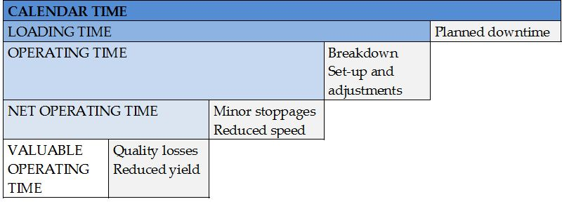
At this point we can define:
|
|
|
|
|
|
Please note that:
|
|
and
|
|

finally
|
|

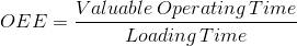
So through a bottom-up approach based on the Six Big Losses model, OEE breaks the performance of equipment into three separate and measurable components: Availability, Performance and Quality.
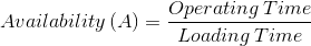
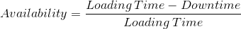
- Availability: it is the percentage of time that equipment is available to run during the total possible Loading Time. Availability is different than Utilization. Availability only includes the time the machine was scheduled, planned, or assigned to run. Utilization regards all hours of the calendar time. Utilization is more effective in capacity planning and analyzing fixed cost absorption. Availability looks at the equipment itself and focuses more on variable cost absorption. Availability can be even calculated as:
|
|
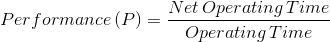
- Performance: it is a measure of how well the machine runs within the Operating Time. Performance can be even calculated as:
|
|

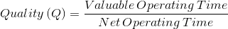
- Quality: it is a measure of the number of parts that meet specification compared to how many were produced. Quality can be even calculated as:
|
|

After the various factors are taken into account, all the results are expressed as a percentage that can be viewed as a snapshot of the current equipment effectiveness.
The value of the OEE is an indication of the size of the technical losses (machine malfunctioning and process) as a whole. The gap between the value of the OEE and 100% indicates the share of technical losses compared to the Loading Time.
The compound effect of Availability, Performance and Quality provides surprising results, as visualized by e.g. Louglin4.
Let’s go through a practical example in the Table 2.2 .
|
Availability |
86,7% |
|
Performance |
93% |
|
Quality |
95% |
|
OEE |
76,6% |
The example in Table 2.2 illustrates the sensitivity of the OEE measure to a low and combined performance. Consequently, it is impossible to reach 100 % OEE within an industrial context. Worldwide studies indicate that the average OEE rate in manufacturing plants is 60%. As pointed out by e.g. Bicheno5 world class level of OEE is in the range of 85 % to 92 % for non-process industry. Clearly, there is room for improvement in most manufacturing plants! The challenge is, however, not to peak on those levels but thus to exhibit a stable OEE at world-class level6.
- 5052 reads
