


Neural networks are a technique based on models of biological brain structure. Artificial Neural Networks (NN), firstly developed by McCulloch and Pitts in 1943, are a mathematical model which wants to reproduce the learning process of human brain1. They are used to simulate and analyse complex systems starting from known input/output examples. An algorithm processes data through its interconnected network of processing units compared to neurons. Consider the Neural Network procedure to be a “black box”. For any particular set of inputs (particular scheduling instance), the black box will give a set of outputs that are suggested actions to solve the problem, even though output cannot be generated by a known mathematical function. NNs are an adaptive system, constituted by several artificial neurons interconnected to form a complex network, those change their structure depending on internal or external information. In other words, this model is not programmed to solve a problem but it learns how to do that, by performing a training (or learning) process which uses a record of examples. This data record, called training set, is constituted by inputs with their corresponding outputs. This process reproduces almost exactly the behaviour of human brain that learns from previous experience.
The basic architecture of a neural network, starting from the taxonomy of the problems faceable with NNs, consists of three layers of neurons: the input layer, which receives the signal from the external environment and is constituted by a number of neurons equal to the number of input variables of the problem; the hidden layer (one or more depending on the complexity of the problem), which processes data coming from the input layer; and the output layer, which gives the results of the system and is constituted by as many neurons as the output variables of the system.
The error of NNs is set according to a testing phase (to confirm the actual predictive power of the network while adjusting the weights of links). After having built a training set of examples coming from historical data and having chosen the kind of architecture to use (among feed-forward networks, recurrent networks), the most important step of the implementation of NNs is the learning process. Through the training, the network can infer the relation between input and output defining the “strength” (weight) of connections between single neurons. This means that, from a very large number of extremely simple processing units (neurons), each of them performing a weighted sum of its inputs and then firing a binary signal if the total input exceeds a certain level (activation threshold), the network manages to perform extremely complex tasks. It is important to note that different categories of learning algorithms exists: (i) supervised learning, with which the network learns the connection between input and output thank to known examples coming from historical data; (ii) unsupervised learning, in which only input values are known and similar stimulations activate close neurons otherwise different stimulations activate distant neurons; and (iii) reinforcement learning, which is a retro-activated algorithm capable to define new values of the connection weights starting from the observation of the changes in the environment. Supervised learning by back error propagation (BEP) algorithm has become the most popular method of training NNs. Application of BEP in Neural Network for production scheduling is in: Dagli et al. (1991)2, Cedimoglu (1993)3, Sim et al. (1994)4, Kim et al. (1995)5.
The mostly NNs architectures used for JSSP are: searching network (Hopfield net) and error correction network (Multi Layer Perceptron). The Hopfield Network (a content addressable memory systems with weighted threshold nodes) dominates, however, neural network based scheduling systems6. They are the only structure that reaches any adequate result with benchmark problems7. It is also the best NN method for other machine scheduling problems8. In Storer et al. (1995)9 this technique was combined with several iterated local search algorithms among which space genetic algorithms clearly outperform other implementations10. The technique’s objective is to minimize the energy function E that corresponds to the makespan of the schedule. The values of the function are determined by the precedence and resource constraints which violation increases a penalty value. The Multi Layer Perceptron (i.e., MLP) consists in a black box of several layers allowing inputs to be added together, strengthened, stopped, non-linearized11, and so on12. The black box has a great no. of knobs on the outside which can be filled with to adjust the output. For the given input problem, the training (network data set is used to adjust the weights on the neural network) is set as optimum target. Training an MLP is NP-complete in general.
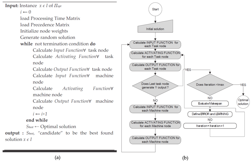
In Figure 5.9 it is possible to see the pseudo-code and the flow chart for the neural networks.
- 3399 reads
