Manufacturing system design: Establish the number of production machines

Available under Creative Commons-ShareAlike 4.0 International License.

Each process designer, when starting the design of a new production system, must ensure that the number of equipments necessary to carry out a given process activity (e.g. metal milling) is sufficient to realize the required volume. Still, the designer must generally ensure that the minimum number of equipment is bought due to elevated investment costs. Clearly, the performance inefficiencies and their propagation became critical, when the purchase of an extra (set of) equipment(s) is required to offset time losses propagation. From a price strategy perspective, the process designer is generally requested to assure the number of requested equipments is effectively the minimum possible for the requested volume. Any not necessary over-sizing results in an extra investment cost for the company, compromising the economical performance.

Typically, the general equation to assess the number of equipments needed to process a demand of products (D) within a total calendar time C _t (usually one year) can be written as follow:

Table 3.1 Equation
$n_{i}= int\left \lceil \frac{D\ast ct_{i}}{C_{t}\ast \vartheta \ast \eta _{i}} \right \rceil+1$

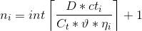
Where:

D is the number of products that must be produced;
ct_i is theoretical cycle time for the equipment i to process a piece of product;
C_t is the number of hours (or minutes) in one year.
ϑ is a coefficient that includes all the external time losses that affect a production system, precluding production.
η _i is the efficiency of the equipment i within the system.

It is therefore possible to define L_t, Loading time, as the percentage of total calendar time C _t that is actually scheduled for operation:

$L_{t}= C_{t}\ast \vartheta$

The Table 3.1 shows that the process designer must consider in his/her analysis three parameters unknown a priori, which influence dramatically the production system sizing and play a key role in the design of the system in order to realize the desired throughput. These parameters affect the total time available for production and the real time each equipment request to realize a piece1, and are respectively:

External time losses, which are considered in the analysis with ϑ;
The theoretical time cycle, which depends upon the selected equipment(s);
The efficiency of the equipment which depends upon the selected equipments and their interactions, in accordance to the specific design.

This list highlights the complexity implicitly involved in a process design. Several forecasts and assumptions may be required. In this sense, it is a good practice to ensure that the ratio in Table 3.2 is always respected for each equipment:

Table 3.2 Equation
$\frac{\frac{D\ast ct_{i}}{L_{t}\ast \eta _{i}}}{n_{i}}< 1$

As a good practice, to ensure Table 3.2 being properly lower than 1 allows to embrace, among others, the variability and uncertainty implicitly embedded within the demand forecast.

In the next paragraph we will analyze the External time losses that must be considered during the design.

1499 reads

You are here

Manufacturing system design: Establish the number of production machines