Reliability basics

The period of regular operation of an equipment ends when any chemical-physical phenomenon, said fault, occurred in one or more of its parts, determines a variation of its nominal performances. This makes the behavior of the device unacceptable. The equipment passes from the state of operation to that of non-functioning.

In Table 4.1 faults are classified according to their origin. For each failure mode an extended description is given.

Table 4.1 Main causes of failure. The table shows the main cases of failure with a detailed description
Failure cause	Description
Stress, shock, fatigue	Function of the temporal and spatial distribution of the load conditions and of the response of the material. The structural characteristics of the component play an important role, and should be assessed in the broadest form as possible, incorporating also possible design errors, embodiments, material defects, etc..
Temperature	Operational variable that depends mainly on the specific characteristics of the material (thermal inertia), as well as the spatial and temporal distribution of heat sources.
Wear	State of physical degradation of the component; it manifests itself as a result of aging phenomena that accompany the normal activities (friction between the materials, exposure to harmful agents, etc..)
Corrosion	Phenomenon that depends on the characteristics of the environment in which the component is operating. These conditions can lead to material degradation or chemical and physical processes that make the component no longer suitable.

To study reliability you need to transform reality into a model, which allows the analysis by applying laws and analyzing its behavior1. Reliability models can be divided into static and dynamic ones.Static models assume that a failure does not result in the occurrence of other faults. Dynamic reliability, instead, assumes that some failures, so-called primary failures, promote the emergence of secondary and tertiary faults, with a cascading effect. In this text we will only deal with static models of reliability.

In the traditional paradigm of static reliability, individual components have a binary status: either working or failed. Systems, in turn, are composed by an integer number n of components, all mutually independent. Depending on how the components are configured in creating the system and according to the operation or failure of individual components, the system either works or does not work.

Let’s consider a generic X_system consisting of nelements. The static reliability modeling implies that the operating status of the i−th component is represented by the state function X_i defined as:

$X_{i}= \left\{\begin{matrix} 1 & if the\, i-th\, component\, works \\ 0 & if the\, i-th \, component\, fails & \end{matrix}\right.$

The state of operation of the system is modeled by the state function Φ(X)

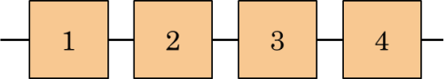
$\Phi \left ( X \right )= \left\{\begin{matrix} 1 & if \: the\: system \: works\\ 0 & if\: the \: system\: fails \end{matrix}\right.$

The most common configuration of the components is the series system. A series system works if and only if all components work. Therefore, the status of a series system is given by the state function:

$\Phi \left ( X \right )= \prod_{i= 1}^{n}X_{i}= \underset{i\in \left \{ 1,2,...,n \right \}}{\textrm{min}}X_{i}$

where the symbol $\prod$ indicates the product of the arguments.

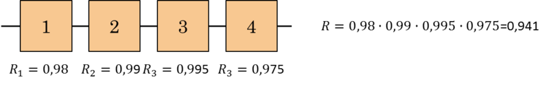
System configurations are often represented graphically with Reliability Block Diagrams (RBDs) where each component is represented by a block and the connections between them express the configuration of the system. The operation of the system depends on the ability to cross the diagram from left to right only by passing through the elements in operation. Figure 4.1 contains the RBD of a four components series system.

Figure 4.1 Reliability block diagram for a four components (1,2,3,4) series system

The second most common configuration of the components is the parallel system. A parallel system works if and only if at least one component is working. A parallel system does not work if and only if all components do not work. So, if Φ−(X) is the function that represents the state of not functioning of the system and X−_i indicates the non-functioning of the i−th element, you can write:

$\overline{\Phi }\left ( X \right )= \prod_{i= 1}^{n}\overline{X}_{i}$

Accordingly, the state of a parallel system is given by the state function:

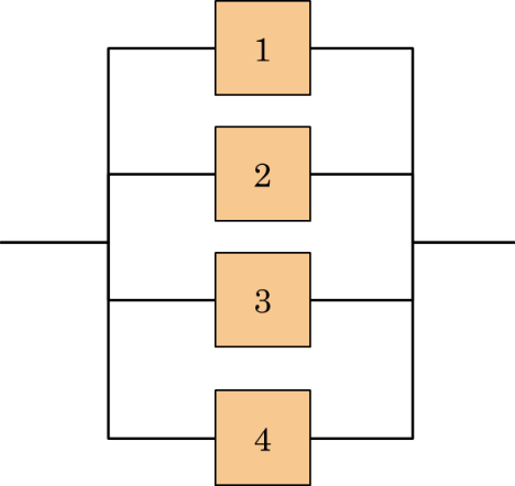
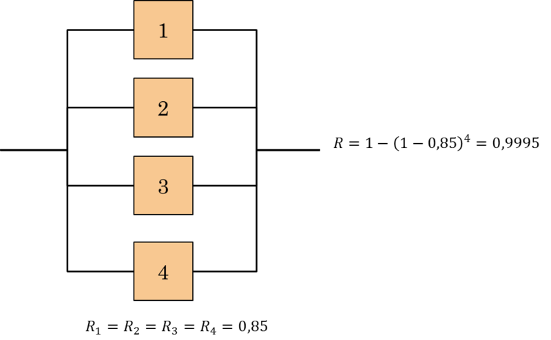
$\Phi \left ( X \right )= 1-\prod_{i= 1}^{n}\left ( 1-X_{i} \right )= \coprod_{i= 1}^{n}X_{i}= \underset{i\in \left \{ 1,2,...,n \right \}}{\textrm{max}}X_{i}$

where the symbol ∐ indicates the complement of the product of the complements of the arguments. Figure 4.2 contains a RBD for a system of four components arranged in parallel.

Figure 4.2 Parallel system

The image represents the RBD of a system of four elements (1,2,3,4) arranged in a reliability parallel configuration.

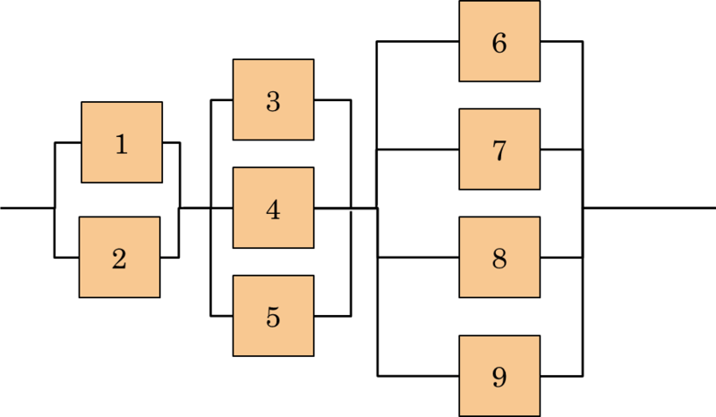
Another common configuration of the components is the series-parallel systems. In these systems, components are configured using combinations in series and parallel configurations. An example of such a system is shown in Figure 4.3.

State functions for series-parallel systems are obtained by decomposition of the system. With this approach, the system is broken down into subsystems or configurations that are in series or in parallel. The state functions of the subsystems are then combined appropriately, depending on how they are configured. A schematic example is shown in Figure 4.4 .

Figure 4.3 Series-parallel system

The picture shows the RBD of a system due to the series-parallel model of 9 elementary units.

Figure 4.4 Calculation of the state function of a series-parallel

Referring to the configuration of Series-parallel system , the state function of the system is calculated by first making the state functions of the parallel of{1,2}, of {3,4,5} and of{6,7,8 , 9}. Then we evaluate the state function of the series of the three groups just obtained.

A particular component configuration, widely recognized and used, is the parallel k out of n. A system k out of n works if and only if at least k of the n components works. Note that a series system can be seen as a system n out of n and a parallel system is a system 1 out of n. The state function of a system k out of n is given by the following algebraic system:

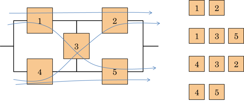
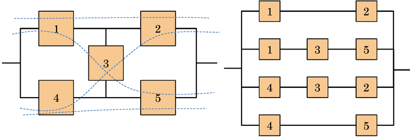
$\Phi \left ( X \right )= \left\{\begin{matrix} 1 & if \sum_{i= 1}^{n}X_{i}\geq k\\ 0 & otherwise \end{matrix}\right.$

The RBD for a system kout of nhas an appearance identical to the RBD schema of a parallel system of n components with the addition of a label "k out of n". For other more complex system configurations, such as the bridge configuration (see Figure 4.5), we may use more intricate techniques such as the minimal path set and the minimal cut set, to construct the system state function.

A Minimal Path Set - MPS is a subset of the components of the system such that the operation of all the components in the subset implies the operation of the system. The set is minimal because the removal of any element from the subset eliminates this property. An example is shown in Figure 4.5.

Figure 4.5 Minimal Path Set

The system on the left contains the minimal path set indicated by the arrows and shown in the right part. Each of them represents a minimal subset of the components of the system such that the operation of all the components in the subset implies the operation of the system.

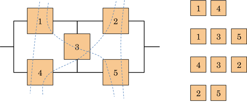
A Minimal Cut Set - MCS is a subset of the components of the system such that the failure of all components in the subset does not imply the operation of the system. Still, the set is called minimal because the removal of any component from the subset clears this property (see Figure 4.6).

Figure 4.6 Minimal Cut Set

The system of the left contains the minimal cut set, indicated by the dashed lines, shown in the right part. Each of them represents a minimum subset of the components of the system such that the failure of all components in the subset does not imply the operation of the system.

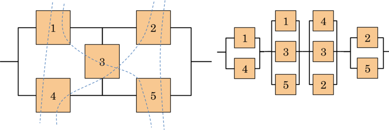
MCS and MPS can be used to build equivalent configurations of more complex systems, not referable to the simple series-parallel model. The first equivalent configuration is based on the consideration that the operation of all the components, in at least a MPS, entails the operation of the system. This configuration is, therefore, constructed with the creation of a series subsystem for each path using only the minimum components of that set. Then, these subsystems are connected in parallel. An example of an equivalent system is shown in Figure 4.7.

Figure 4.7 Equivalent configurations with MPS

You build a series subsystem for each MPS. Then such subsystems are connected in parallel.

The second equivalent configuration, is based on the logical principle that the failure of all the components of any MCS implies the fault of the system. This configuration is built with the creation of a parallel subsystem for each MCS using only the components of that group. Then, these subsystems are connected in series (see Figure 4.8).

Figure 4.8 Equivalent configurations with MCS

You build a subsystem in parallel for each MCS. Then the subsystems are connected in series.

After examining the components and the status of the system, the next step in the static modeling of reliability is that of considering the probability of operation of the component and of the system.

The reliability R_i of the i−th component is defined by:

$R_{i}= P\left ( X_{i}= 1 \right )$

while the reliability of the system R is defined as in Table 4.2 :

Table 4.2 Equation
$R= P\left ( \Phi \left ( X \right )= 1 \right )$

The methodology used to calculate the reliability of the system depends on the configuration of the system itself. For a series system, the reliability of the system is given by the product of the individual reliability (law of Lusser, defined by German engineer Robert Lusser in the 50s):

Table 4.3 Equation
$R= \prod_{i= 1}^{n}R_{i}\; since\; R= P\left ( \bigcap_{i= 1}^{n}\left ( X_{i}= 1 \right ) \right )= \prod_{i= 1}^{n}P\left ( X_{i}= 1 \right )= \prod_{i= 1}^{n}R_{i}$

For an example, see Figure 4.9 .

Figure 4.9 serial system consisting of 4 elements with reliability equal to 0.98, 0.99, 0.995 and 0.975

The reliability of the whole system is given by their product: R = 0.98 ⋅ 0.99 ⋅ 0.995 ⋅ 0.975 = 0.941

For a parallel system, reliability is:

Table 4.4 Equation
$R= 1-\prod_{i= 1}^{n}\left ( 1-R_{i} \right )= \coprod_{i= 1}^{n}R_{i}$

In fact, from the definition of system reliability and by the properties of event probabilities, it follows:

$R= P\left ( \bigcup_{i= 1}^{n}\left ( X_{i}= 1 \right ) \right )= 1-P\left ( \bigcap_{i=1}^{n}\left ( X_{i=0} \right ) \right )=1-\prod_{i=1}^{n}P\left ( X_{i}=0 \right )== 1-\prod_{i=1}^{n}\left [ 1-P\left ( X_{i}=1 \right ) \right ]-\prod_{i=1}^{n}\left ( 1-R_{i} \right )= \coprod_{i=1}^{n}R_{i}$

In many parallel systems, components are identical. In this case, the reliability of a parallel system with n elements is given by:

$R= 1- \left ( 1-R_{i} \right )^{n}$

Figure 4.10 A parallel system consisting of 4 elements with the same reliability of 0.85

The system reliability s given by their co-product: 1−(1−0.85)⁴=0.9995.

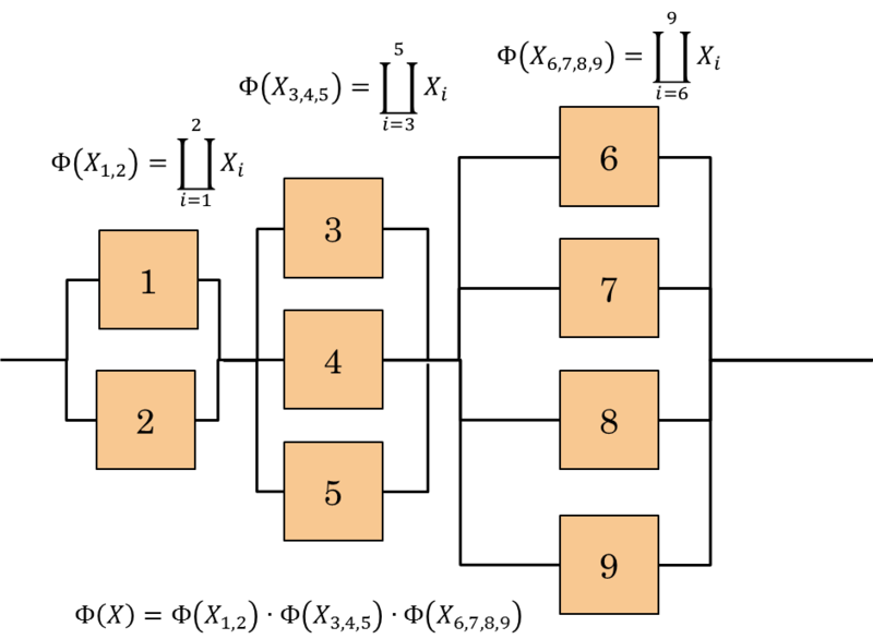
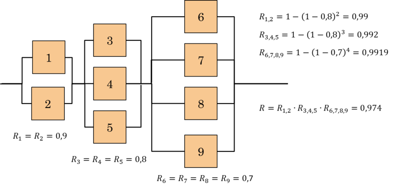
For a series-parallel system, system reliability is determined using the same approach of decomposition used to construct the state function for such systems. Consider, for instance, the system drawn in Figure 4.11 , consisting of 9 elements with reliability R₁=R₂=0.9; R₃=R₄=R₅=0.8 and R₆=R₇=R₈=R₉=0.7. Let’s calculate the overall reliability of the system.

Figure 4.11 The system consists of three groups of blocks arranged in series

Each block is, in turn, formed by elements in parallel. First we must calculate R_1,2=1−(1−0.8)²=0.99. So it is possible to estimated R_3,4,5=1−(1−0.8)³=0.992. Then we must calculate the reliability of the last parallel block R_6,7,8,9=1−(1−0.7)⁴=0.9919. Finally, we proceed to the series of the three blocks: R=R_1,2∙R_3,4,5∙R_6,7,8,9=0.974.

To calculate the overall reliability, for all other types of systems which can’t be brought back to a series-parallel scheme, it must be adopted a more intensive calculation approach2 that is normally done with the aid of special software.

Reliability functions of the system can also be used to calculate measures of reliability importance.

These measurements are used to assess which components of a system offer the greatest opportunity to improve the overall reliability. The most widely recognized definition of reliability importance I'_i of the components is the reliability marginal gain, in terms of overall system rise of functionality, obtained by a marginal increase of the component reliability:

$I'\: _{i}=\frac{\partial R}{\partial R_{i}}$

For other system configurations, an alternative approach facilitates the calculation of reliability importance of the components. Let R(1_i)be the reliability of the system modified so that R_i=1and R(0_i)be the reliability of the system modified withR_i=0, always keeping unchanged the other components. In this context, the reliability importance I_i is given by:

$I_{i}= R\left ( 1_{i} \right )-R\left ( 0_{i} \right )$

In a series system, this formulation is equivalent to writing:

$I_{i}= \prod_{\begin{matrix} j=1\\ j\neq i \end{matrix}}^{n}R_{j}$

Thus, the most important component (in terms of reliability) in a series system is the less reliable. For example, consider three elements of reliability
R₁=0.9, R₂=0.8 e R₃=0.7. It is therefore:
I₁=0.8∙0.7=0.56, I₂=0.9∙0.7=0.63 and I₃=0.9⋅0.8=0.72 which is the higher value.

If the system is arranged in parallel, the reliability importance becomes as follows:

Table 4.5 Equation
$I_{i}= \prod_{\begin{matrix} j=1\\ j\neq i \end{matrix}}^{n}\left ( 1-R_{j} \right )$

It follows that the most important component in a parallel system is the more reliable. With the same data as the previous example, this time having a parallel arrangement, we can verify Table 4.5 for the first item: I₁=R(1₁)−R(0₁)=
[1−(1−1)⋅(1−0.8)∙(1−0.7)]−[1−(1−0)⋅(1−0.8)∙(1−0.7)]
=1−0−1+(1−0.8)∙(1−0.7)=(1−0.8)∙(1−0.7).

For the calculation of the reliability importance of components belonging to complex systems, which are not attributable to the series-parallel simple scheme, reliability of different systems must be counted. For this reason the calculation is often done using automated algorithms.

3027 reads

You are here

Reliability basics