The mixed-model JIT scheduling problem

Available under Creative Commons-ShareAlike 4.0 International License.

The leveling problem in JIT operations research literature was formalized in 1983 as the “mixed-model just-in-time scheduling (or sequencing) problem” (MMJIT)1, along with its first solution approach, the “Goal Chasing Method” (GCM I) heuristic.

Some assumptions are usually made to approach this problem2. The most common are:

no variability; the problem is defined in a deterministic scenario;
no details on the process phases: the process is considered as a black box, which transforms raw materials in finished products;
zero setup times (or setup times are negligible);
demand is constant and known;
production lead time is the same for each product.

Unfortunately, the problem with these assumptions virtually never occurs in industry. However, the problem is of mathematical interest because of its high complexity (in a theoretical mathematical sense). Because researchers drew their inspiration from the literature and not from industry, on MMJIT far more was published than practiced.

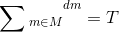
The objective of a MMJIT is to obtain a leveled production. This aim is formalized in the Output Rate Variation (ORV) objective function (OF)3, 4. Consider a M set of m product models, each one with a d_m demand to be produced during a specific period (e.g., 1 day or shift) divided into T production cycles, with

${\sum { }_{m \in M}}^{dm}=T$

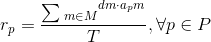
Each product type m consists of different components p belonging to the set P. The production coefficients a_pm specify the number of units of part p needed in the assembly of one unit of product m. The matrix of coefficients A = (a_pm) represents the Bill Of Material (BOM). Given the total demand for part p required for the production of all m models in the planning horizon, the target demand rate r_p per production cycle is calculated as follows:

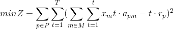
$r_p=\frac{{\sum { }_{m \in M}}^{dm\cdot a_pm}}{T} ,\forall p\in P$

Given a set of binary variables x_mt which represent whether a product m will be produced in the t cycle, the problem is modeled as follows5:

$minZ=\sum _{p\in P}\sum_{t=1}^T (\sum_{m\in M}\sum_{t=1}^t x_mt\cdot a_{pm}-t\cdot r_p)^{2}$

subject to

$\sum{ }_{m\in M^{xmt}}=1,\forall t=1,...,T$

$\sum_{t=1}^T x_{mt}=d_m,\forall m\in M$

$x_{mt}\in \left \{ 0,1 \right \}, \forall m \in M;t=1,...,T$

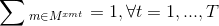
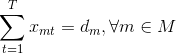
The first and second group of constraints indicate that for each time t exactly one model will be produced and that the total demand d_m for each model will be fulfilled by the time T. More constraints can be added if required, for instance in case of limited storage space.

A simplified version of this problem, labeled “Product Rate Variation Problem” (PRV) was studied by several authors6, 7, 8 ], although it was found it is not sufficient to cope with the variety of production models of modern assembly lines9. Other adaptations of this problem were proposed along the years; after 2000, when some effective solving algorithms were proposed10, the literature interest moved on to the MMJIT scheduling problem with setups11. In this case, a dual OF is used12: the first part is the ORV/PRV standard function, while the second is simply:

$minS=1+\sum_{t=2}^T s_t$

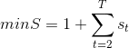
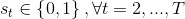
In this equation, s_t = 1 if a setup is required in position t; while s_t ₌ 0, if no setup is required. The assumptions of this model are:

an initial setup is required regardless of sequence; this is the reason for the initial “1” and the t index follows on “2”;

the setup time is standard and it is not dependent from the product type;

the setup number and setup time are directly proportional each other.

The following sets of bounds must be added in order to shift s_t from “0” to “1” if the production switches from a product to another:

$x_{m(t-1)}-x_{mt}\leq s_t,\forall t=2,...,T,\forall m \in M$

$s_t \in \left \{ 0,1 \right \}, \forall t =2,...,T$

Being a multi-objective problem, the MMJIT with setups has been approached in different ways, but it seems that no one succeeded in solving the problem using a standard mathematical approach. A simulation approach was used in13. Most of the existing studies in the literature use mathematical representations, Markov chains or simulation approaches. Some authors14, 15 ] reported that the following parameters may vary within the research carried out in the recent years, as shown in Table 2.1 below.

1784 reads

You are here

The mixed-model JIT scheduling problem