Representation of scheduling instances

Available under Creative Commons-ShareAlike 4.0 International License.

The possible representation of a JS problem could be done through a Gantt chart or through a Network representation.

Gantt (1916) created innovative charts for visualizing planned and actual production1. According to Cox et al. (1992), a Gantt chart is „the earliest and best known type of control chart especially designed to show graphically the relationship between planned performance and actual performance”2. Gantt designed his charts so that foremen or other supervisors could quickly know whether production was on schedule, ahead of schedule or behind schedule. A Gantt chart, or bar chart as it is usually named, measures activities by the amount of time needed to complete them and use the space on the chart to represent the amount of the activity that should have been done in that time3.

A Network representation was first introduced by Roy and Sussman4. The representation is based on “disjunctive graph model”5. This representation starts from the concept that a feasible and optimal solution of JSP can originate from a permutation of task’s order. Tasks are defined in a network representation through a probabilistic model, observing the precedence constraints, characterized in a machine occupation matrix M and considering the processing time of each tasks, defined in a time occupation matrix T.

$M=\begin{pmatrix} M_{11}&\cdots&M_{1n} \\ \vdots&\ddots&\vdots \\ M_{n1}&\cdots&M_{nn} \end{pmatrix} ; \begin{pmatrix} \tau \left ( M_{11} \right )&\cdots&\tau \left ( M_{1n} \right ) \\ \vdots&\ddots&\vdots \\ \tau \left ( M_{n1} \right )&\cdots&\tau \left ( M_{nn} \right ) \end{pmatrix}$

JS processes are mathematically described as disjunctive graph G = (V, C, E). The descriptions and notations as follow are due to Adams et. al.6, where:

V is a set of nodes representing tasks of jobs. Two additional dummy tasks are to be considered: a source(0) node and a sink(*) node which stand respectively for the Source (S) task $\tau_0=0$ , necessary to specify which job will be scheduled first, and an end fixed sink where schedule ends $(T)\tau *=0$ ;
C is the set of conjunctive arcs or direct arcs that connect two consecutive tasks belonging to the same job chain. These represent technological sequences of machines for each job;
$E=\cup _{r=1}^{m}D_r$ , where D_r is a set of disjunctive arcs or not-direct arcs representing pair of operations that must be performed on the same machine M_r.

Each job-tasks pair (i,j) is to be processed on a specified machine M(i,j) for T(i,j) time units, so each node of graph is weighted with j operation’s processing time. In this representation all nodes are weighted with exception of source and sink node. This procedure makes always available feasible schedules which don’t violate hard constraints7 - . A graph representation of a simple instance of JSP, consisting of 9 operations partitioned into 3 jobs and 3 machines, is presented in Figure 5.1. Here the nodes correspond to operations numbered with consecutive ordinal values adding two fictitious additional ones:S = “source node” and T = “sink node”. The processing time for each operation is the weighted value τ_ij attached to the corresponding node,v∈V, and for the special nodes, $\tau _0=\tau *=0$ .

Let s_v be the starting time of an operation to a node v. By using the disjunctive graph notation, the JSPP can be formulated as a mathematical programming model as follows:

Minimize s_* subject to:

${S_{w}}-{S_{v}}\geq {}\tau _{v}}\left ( v,w \right )\in C$

$s_{v}\geq \textrm{0v}\in \textrm{V}$

${s_{w}}-{s_{v}}\geq \tau _{v}\vee s_{v}-{s_{w}}\geq \tau _{w}\left ( \textrm{v,w} \right )\in D_{r}$

Figure 5.1 Disjunctive graph representation.

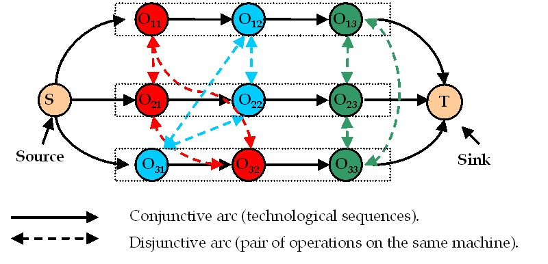
In Figure 5.1 There are disjunctive arcs between every pair of tasks that has to be processed on the same machine (dashed lines) and conjunctive arcs between every pair of tasks that are in the same job (dotted lines). Omitting processing time, the problem specification is $O=\left \{ oij, (i,j)\in \left \{ 1,2,3 \right \}^2 \right \}, J= \left \{ J_i=\left \{ oij \right \}, (i,j)= 1,2,3 \right \},$ $M=\left \{ M_j=\left \{ oij \right \}, (i,j)= 1,2,3 \right \}$ . Job notation is used.

s_* is equal to the completion time of the last operation of the schedule, which is therefore equal to C_max. The first inequality ensures that when there is a conjunctive arc from a node v to a node w, w must wait of least τ_v time after v is started, so that the predefined technological constraints about sequence of machines for each job is not violated. The second condition ensures time to start continuities. The third condition affirms that, when there is a disjunctive arc between a node v and a node w, one has to select either v to be processed prior to w (and w waits for at least τ_v time period) or the other way around, this avoids overlap in time due to contemporaneous operations on the same machine.

In order to obtain a scheduling solution and to evaluate makespan, we have to collect all feasible permutations of tasks to transform the undirected arcs in directed ones in such a way that there are no cycles.

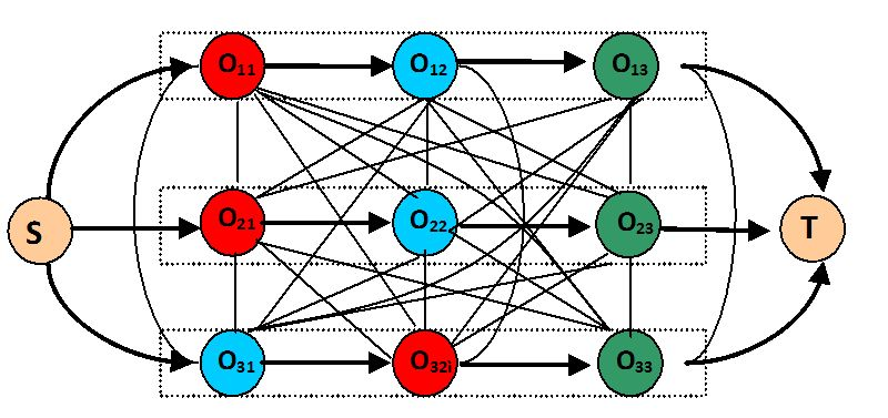
The total number of nodes, n=(|O|+2)− fixed by taking into account the total number of tasks |O|, is properly the total number of operations with more two fictitious ones. While the total number of arcs, in job notation, is fixed considering the number of tasks and jobs of instance:

$arcs=\binom{n}{2}+2\times \mid J\left.\begin{matrix}\\ \\ \end{matrix}\right|=\frac{\left ( \mid O\mid \right )\times \left \{ \left ( \mid O\mid \right ) -1\right \}}{2}+2\times \mid J\left.\begin{matrix} \\ \\ \end{matrix}\right|$

The number of arcs defines the possible combination paths. Each path from source to sink is a candidate solution for JSSP. The routing graph is reported in Figure 5.2:

Figure 5.2 Problem routing representation.

2043 reads

You are here

Representation of scheduling instances