


In accordance with the proposed method (§ 3.5) we show how availability losses propagate in the system and to assess the effect of buffer capacity on OEE through the simulation. We focuses on the insulating and packaging working stations. Technical data about availability of equipment are: mean time between failure for insulating is 20000 sec while for packaging is 30000 sec; mean time between repair for insulating is 10000 sec while for packaging is 30000 sec. The cycle time of the working stations are the same equal to 2800 sec for coil. The quality rates are set to 1. Idling, minor stoppages and reduced speed are not considered and set to 0.
Considering equipment isolated from the system the OEE for the single machine is equal to its availability; in particular, relating to previous data, machines have an OEE equal to 0,67 and 0,5 respectively for insulating and packaging. The case points out how the losses due to major stoppage spread to other station in function of buffer capacity dimension.
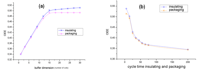
A simulation has been run to study the effect of buffer capacity in this case. Capacity of buffer downstream of insulating has been changed from 0 to 30 coils for different simulations. The results of simulations are shown in Figure 3.15a. The OEE for both machines is equal to 0,33 with no buffer capacity. This results is the composition of availability of insulating and packaging (0,67 x 0,5) as expected. The OEEs increase in function of buffer dimension that avoids the propagation of major stoppage and availability losses propagation. Also the OTE is equal to 0,33 that is, according to formulation in (1) and as previously explained, equal to OEE of the last station but assessed in the system.
Insulating and packaging increase rapidly OEEs since a structural limits of buffer capacity of 15 coils; from this value OEEs of two stations converge on value of 0,5. The upstream insulating station, that has an availability greater than packaging, has to adapt itself to real cycle time of packaging that is the bottleneck station.
It’s important to point out that in performance monitoring of manufacturing plant the propagation of the previous losses is often gathered as performance losses (reduced speed or minor stoppage) in absence of specific data collection relating to major stoppage due to absence of material flow. So, if we consider also all other efficiency looses ignored in this sample, we can understand how much could be difficult to identify the real impact of this kind of efficiency losses monitoring the real system. Moreover simulation supports in system design in order to dimension buffer capacity (e.g. in this case structural limit for OEE is reached for 16 coils). Moreover through simulation it is possible to point out that the positive effect of buffer is reduced with an higher cycle time of machine as shown in Figure 3.15b.
- 2492 reads
