


If we are on a pic-nic and peer into our cake bitten by a colony of ants, moving in a tidy way and caring on a lay-out that is the optimal one in view of stumbling-blocks and length, we discover how remarkable is nature and we find its evolution as the inspiring source for investigations on intelligence operation scheduling techniques1. Natural ants are capable to establish the shortest route path from their colony to feeding sources, relying on the phenomena of swarm intelligence for survival. They make decisions that seemingly require an high degree of co-operation, smelling and following a chemical substance (i.e. pheromone2 - ) laid on the ground and proportional to goodness load that they carry on (i.e. in a scheduling approach, the goodness of the objective function, reported to makespan in this applicative case).
The same behaviour of natural ants can be overcome in an artificial system with an artificial communication strategy regard as a direct metaphoric representation of natural evolution. The essential idea of an ACO model is that „good solutions are not the result of a sporadic good approach to the problem but the incremental output of good partial solutions item. Artificial ants are quite different by their natural progenitors, maintaining a memory of the step before the last one3. Computationally, ACO4are population based approach built on stochastic solution construction procedures with a retroactive control improvement, that build solution route with a probabilistic approach and through a suitable selection procedure by taking into account: (a) heuristic information on the problem instance being solved; (b) (mat-made) pheromone amount, different from ant to ant, which stores up and evaporates dynamically at run-time to reflect the agents’ acquired search training and elapsed time factor.
The initial schedule is constructed by taking into account heuristic information, initial pheromone setting and, if several routes are applicable, a self-created selection procedure chooses the task to process. The same process is followed during the whole run time. The probabilistic approach focused on pheromone. Path’s attractive raises with path choice and probability increases with the number of times that the same path was chosen before5. At the same time, the employment of heuristic information can guide the ants towards the most promising solutions and additionally, the use of an agent’s colony can give the algorithm: (i) Robustness on a fixed solution; (ii) Flexibility between different paths.
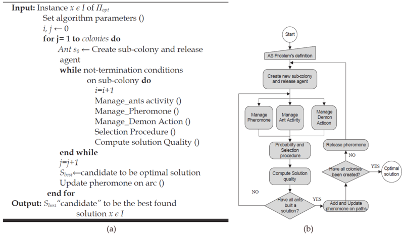
The approach focuses on co-operative ant colony food retrieval applied to scheduling routing problems. Colorni et al, basing on studies of Dorigo et al.6, were the first to apply Ant System (AS) to job scheduling problem7 and dubbed this approach as Ant Colony Optimization (ACO). They iteratively create route, adding components to partial solution, by taking into account heuristic information on the problem instance being solved (i.e. visibility) and “artificial” pheromone trials (with its storing and evaporation criteria). Across the representation of scheduling problem like acyclic graph, see Figure 1.2, the ant’s rooting from source to food is assimilated to the scheduling sequence. Think at ants as agents, nodes like tasks and arcs as the release of production order. According to constraints, the ants perform a path from the row material warehouse to the final products one.
Constraints are introduced hanging from jobs and resources. Fitness is introduced to translate how good the explored route was. Artificial ants live in a computer realized world. They have an overview of the problem instance they are going to solve across a visibility factor. In the Job Shop side of ACO implementation the visibility has chosen tied with the run time of the task (Table). The information was about the inquired task’s (i.e., j) completion time Ctimej and idle time Itimej from the previous position (i.e., i):

|
The colony is composed of a fixed number of agents ant=1,…, n. A probability is associated to each feasible movement (Sant(t)) and a selection procedure (generally based on RWS or Tournament procedure) is applied.
 is the probability that at time
t the generic agent ant chooses edge i→j as next routing path; at time t each ant chooses the next operation where it will be at time t+1. This value is valuated through visibility (η) and pheromone (τ) information. The probability value (Table) is associated to a fitness into selection step.
is the probability that at time
t the generic agent ant chooses edge i→j as next routing path; at time t each ant chooses the next operation where it will be at time t+1. This value is valuated through visibility (η) and pheromone (τ) information. The probability value (Table) is associated to a fitness into selection step.
![P_{ij}^{ant}\left ( t \right )=\begin{Bmatrix} \frac{\left [\tau _{ij}\left ( t \right ) \right ]^{\alpha }\left [ \eta _{ij}\left ( t \right ) \right ]^{\beta }}{\sum_{h\in S_{ant}\left ( t \right )}^{ }\left [ \tau _{ih}\left ( t \right ) \right ]^{\alpha }\left [ \eta _{ih}\left ( t \right ) \right ]^{\beta }_{i}}&\textrm{if j }\in S_{ant}\left ( t \right ) \\ 0 &\textrm{ otherwise} \end{Bmatrix}](/system/files/resource/18/18769/27149/media/eqn-img_25.gif)
|
Where: represents the intensity of trail on connection
 at time
  . Set
the intensity of pheromone at iteration
. Set
the intensity of pheromone at iteration  to a general small positive constant in order to ensure the avoiding of
local optimal solution; α and β are user’s defined values tuning the relative importance of the pheromone vs. the heuristic time-distance coefficient. They have to be chosen
to a general small positive constant in order to ensure the avoiding of
local optimal solution; α and β are user’s defined values tuning the relative importance of the pheromone vs. the heuristic time-distance coefficient. They have to be chosen (in order to assure a right selection pressure).
For each cycle the agents of the colony are going out of source in search of food. When all colony agents have constructed a complete path, i.e. the sequence of feasible order of visited nodes, a pheromone update rule is applied (Table):

|
Besides ants’ activity, pheromone trail evaporation has been included trough a coefficient representing pheromone vanishing during elapsing time. These parameters imitate the
natural world decreasing of pheromone trail intensity over time. It implements a useful form of forgetting. It has been considered a simple decay coefficient (i.e., ) that works on total laid pheromone level between time t and t+1.
The laid pheromone on the inquired path is evaluated taking into consideration how many agents chose that path and how was the objective value of that path (Table). The weight of the solution goodness is the makespan (i.e., Lant). A constant of pheromone updating (i.e., Q), equal for all ants and user, defined according to the tuning of the algorithm, is introduced as quantity of pheromone per unit of time (Table). The algorithm works as follow. It is computed the makespan value for each agent of the colony (Lant(0)), following visibility and pheromone defined initially by the user (τij(0)) equal for all connections. It is evaluated and laid, according to the disjunctive graph representation of the instance in issue, the amount of pheromone on each arc (evaporation coefficient is applied to design the environment at the next step).
|
|
Visibility and updated pheromone trail fixes the probability (i.e., the fitness values) of each node (i.e., task) at each iteration; for each cycle, it is evaluated the output of the objective
function (Lant(t)). An objective function value is optimised accordingly to partial good solution. In this improvement, relative importance is
given to the parameters α and β. Good elements for choosing these two parameters are: (which means low level of
  ) and little value of
 while ranging β in a larger range
- 12785 reads
