


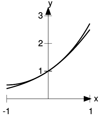
If you calculate  on your calculator, you’ll find that it’s very
close to 1.1. This is because the tangent line at x= 0 on the graph of
on your calculator, you’ll find that it’s very
close to 1.1. This is because the tangent line at x= 0 on the graph of  has a slope of 1 (
 at x= 0), and the tangent line is a good approximation to the exponential curve as long as we don’t get too far away from
the point of tangency.
at x= 0), and the tangent line is a good approximation to the exponential curve as long as we don’t get too far away from
the point of tangency.
How big is the error? The actual value of  is 1.10517091807565
..., which differs from 1.1 by about 0.005. If we go farther from the point of tangency, the approximation gets worse. At x= 0.2, the error
is 1.10517091807565
..., which differs from 1.1 by about 0.005. If we go farther from the point of tangency, the approximation gets worse. At x= 0.2, the error

 , and the tangent line at x = 0.
is about 0.021, which is about four times bigger. In other words, doubling x seems to roughly quadruple the error, so the error is proportional to  ; it seems to be about
  /2. Well, if we want a handy-dandy, super-accurate estimate of
  for small values of x, why not just account for this error. Our new and improved estimate
is
for small values of x, why not just account for this error. Our new and improved estimate
is
 ≈1 + x+
for small values of x.
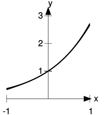
b / The function  , and the approximation 1 + x
+
, and the approximation 1 + x
+  /2.
/2.
Figure b shows that the approximation is now extremely good for sufficiently small values of x. The difference is that whereas 1 + x matched both the y-intercept and the slope
of the curve, 1 + x+  /2 matches the
curvature as well. Recall that the second derivative is a measure of curvature. The second derivatives of the function and its approximation are
/2 matches the
curvature as well. Recall that the second derivative is a measure of curvature. The second derivatives of the function and its approximation are 
We can do even better. Suppose
c / The function  , and the approximation
 ≈ 1 + x+
Figure c shows the result. For a significant range of xvalues close to zero, the approximation is now so good that we can’t even see the difference between the two functions on the
graph.
On the other hand, figure d shows that the cubic approximation for somewhat larger negative and positive values of xis poor — worse, in fact, than the linear approximation, or even the
constant approximation  = 1. This is to be expected, because any
polynomial will blow up to either positive or negative infinity as x approaches negative infinity, whereas the function
= 1. This is to be expected, because any
polynomial will blow up to either positive or negative infinity as x approaches negative infinity, whereas the function  is supposed to get very close to zero for large negative x. The idea here is that derivatives are
local things: they only measure the properties of a function very close to the point at which they’re evaluated, and they don’t necessarily tell us anything about
points far away.
is supposed to get very close to zero for large negative x. The idea here is that derivatives are
local things: they only measure the properties of a function very close to the point at which they’re evaluated, and they don’t necessarily tell us anything about
points far away.

 , on a
wider scale.
, on a
wider scale.
 . But what is the pattern here that would
allows us to gure out, say, the fourth-order and fth-order terms that were swept under the rug with the symbol \. . . "? Let's do the fth-order term as an example. The point of adding in a
fth-order term is to make the fth derivative of the approximation equal to the fth derivative of
. But what is the pattern here that would
allows us to gure out, say, the fourth-order and fth-order terms that were swept under the rug with the symbol \. . . "? Let's do the fth-order term as an example. The point of adding in a
fth-order term is to make the fth derivative of the approximation equal to the fth derivative of  , which is 1. The rst, second, . . . derivatives of x5 are
The notation for a product like 1 ·2 ·...·n is n!, read “n factorial.” So to get a term for our polynomial whose
fifth derivative is 1, we need  /5!. The
result for the infinite series is
/5!. The
result for the infinite series is 
where the special case of 0! = 1 is assumed. 1 This infinite
series is called the Taylor series for  , evaluated around x= 0, and it’s true, although I haven’t proved it, that this particular Taylor series always converges
to
, evaluated around x= 0, and it’s true, although I haven’t proved it, that this particular Taylor series always converges
to  , no matter how far x is from zero.
In general, the Taylor series around x= 0 for a function y is 
where the condition for equality of the nth order derivative is
Here the notation  means that the derivative is to be evaluated
at x= 0.
means that the derivative is to be evaluated
at x= 0.
A Taylor series can be used to approximate other functions besides  , and when you ask your calculator to evaluate a function such as a sine or a cosine, it may actually be using a Taylor series to
do it. Taylor series are also the method Inf uses to calculate most expressions involving infinitesimals. In example 13 on page 29, we saw that when Inf was asked to calculate 1/(1
−d), where d was infinitesimal, the result was the geometric series:
, and when you ask your calculator to evaluate a function such as a sine or a cosine, it may actually be using a Taylor series to
do it. Taylor series are also the method Inf uses to calculate most expressions involving infinitesimals. In example 13 on page 29, we saw that when Inf was asked to calculate 1/(1
−d), where d was infinitesimal, the result was the geometric series:
: 1/(1-d)
1+d+d^2+d^3+d^4
These are also the the first five terms of the Taylor series for the function y= 1/(1 −x), evaluated around x= 0. That is, the geo- metric series 1
+ x+  +
+  + ... is really just one special example of a Taylor series,
as demonstrated in the following example.
+ ... is really just one special example of a Taylor series,
as demonstrated in the following example.
Example 83
Find the Taylor series of y= 1/(1 −x) around x= 0.
Rewriting the function as  and applying the chain
rule, we have
and applying the chain
rule, we have
The pattern is that the nth derivative is n!. The Taylor series therefore has  = n!/n! = 1:
If you flip back to Tests for convergence and compare the rate of convergence of the geometric series for x = 0.1 and 0.5, you’ll see that the sum converged much more quickly for x= 0.1 than for x= 0.5. In general, we expect that any Taylor series will converge more quickly when xis smaller. Now consider what happens at x= 1. The series is now 1 + 1 + 1 + ..., which gives an infinite result, and we shouldn’t have expected any better behavior, since attempting to evaluate 1/(1 −x) at x =1 gives division by zero. For x>1, the results become nonsense. For example, 1/(1 −2) = −1, which is finite, but the geometric series gives 1 + 2 + 4 + ..., which is infinite.
In general, every function’s Taylor series around x= 0 converges for all values of xin the range defined by |x|<r, where ris some number, known as the radius of convergence. Also, if the function is defined by putting together other functions that are well behaved (in the sense of converging to their own Taylor series in the relevant region), then the Taylor series will not only converge but converge to the correctvalue. For the function ex, the radius happen to be infinite, whereas for 1/(1 −x) it equals 1. The following example shows a worst-case scenario.
Example 84
The function  , shown in figure e
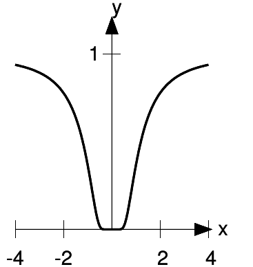
e / The function  never converges to its Taylor series.
never converges to its Taylor series, except at x = 0. This is because the Taylor series for this function, evaluated around x = 0 is exactly zero! At x = 0, we have y = 0, dy / dx = 0,
 = 0, and so on for every derivative. The zero function
matches the function y (x) and all its derivatives to all orders, and yet is useless as an approximation to y (x). The radius of convergence of the Taylor series is infinite, but it doesn’t
give correct results except at x = 0. The reason for this is that y was built by composing two functions, w (x) = −1/
= 0, and so on for every derivative. The zero function
matches the function y (x) and all its derivatives to all orders, and yet is useless as an approximation to y (x). The radius of convergence of the Taylor series is infinite, but it doesn’t
give correct results except at x = 0. The reason for this is that y was built by composing two functions, w (x) = −1/ and y (w) =
  . The function w is badly behaved at x = 0 because it blows up there. In particular, it doesn’t have a well-defined Taylor
series at x = 0
. The function w is badly behaved at x = 0 because it blows up there. In particular, it doesn’t have a well-defined Taylor
series at x = 0
Example 85
Find the Taylor series of y= sin x, evaluated around x= 0.
The first few derivatives are
We can see that there will be a cycle of sin, cos, −sin, and −cos, repeating indefinitely. Evaluating these derivatives at x= 0, we have 0, 1, 0,−1, . . . . All the even-order terms of the series are zero, and all the odd- order terms are ±1/n!. The result is
The linear term is the familiar small- angle approximation sin x≈x.
The radius of convergence of this series turns out to be infinite. Intuitively the reason for this is that the factorials grow extremely rapidly, so that the successive terms in the series eventually start diminish quickly, even for large values of x.
Example 86
Suppose that we want to evaluate a limit of the form

where u(0) = v(0) = 0. L’Hoˆ pital’s rule tells us that we can do this by taking derivatives on the top and bottom to form
u'/v', and that, if necessary, we can do more than one derivative, e.g.,u"/v". This was proved using
the mean value theorem. But if u and vare both functions that converge to their Taylor series, then it is much easier to see why this works. For ex- ample, suppose that
their Taylor series both have vanishing constant and linear terms, so that u= a  + ...and v= b
 + .... Then u"= 2a+ ..., and
v" = 2b+ ....
+ .... Then u"= 2a+ ..., and
v" = 2b+ ....
A function’s Taylor series doesn’t have to be evaluated around x=0. The Taylor series around some other center x= cis given by
 where
where
To see that this is the right generalization, we can do a change of variable, defining a new function g(x) = f(x−c). The radius of convergence is to be measured from the center crather than from 0.
Example 87
Find the Taylor series of ln x, evaluated around x= 1.
Evaluating a few derivatives, we get
Note that evaluating these at x= 0 wouldn’t have worked, since division by zero is undefined; this is because ln xblows up to negative infinity at x = 0. Evaluating them at x= 1, we find that the nthderivative equals ±(n−1)!, so the coefficients of the Taylor series are ±(n−1)!/n! = ±1/n, except for the n= 0 term, which is zero because ln 1 = 0. The resulting series is
We can predict that its radius of convergence can’t be any greater than 1, because ln xblows up at 0, which is at a distance of 1 from 1.
- 4539 reads
