The second derivative

Available under Creative Commons-ShareAlike 4.0 International License.

I described how Galileo and Newton found that an object subject to an external force, starting from rest, would have a velocity $\dot{x}$ that was proportional to , and a position that varied like t^2 . The proportionality constant for the velocity is called the acceleration, , so that $\dot{x}=at$ and x=at^2/2 . For example, a sports car accelerating from a stop sign would have a large acceleration, and its velocity at a given time would therefore be a large number. The acceleration can be thought of as the derivative of the derivative of , written $\ddot{x}$ , with two dots. In our example, $\ddot{x}=a$ . In general, the acceleration doesn't need to be constant. For example, the sports car will eventually have to stop accelerating, perhaps because the backward force of air friction becomes as great as the force pushing it forward. The total force acting on the car would then be zero, and the car would continue in motion at a constant speed.

Example

Suppose the pilot of a blimp has just turned on the motor that runs its propeller, and the propeller is spinning up. The resulting force on the blimp is therefore increasing steadily, and let’s say that this causes the blimp to have an acceleration $\ddot{x}=3t$ , which increases steadily with time. We want to find the blimp’s velocity and position as functions of time.

For the velocity, we need a polynomial whose derivative is . We know that the derivative of t^2 is , so we need to use a function that’s bigger by a factor of $3/2:\dot{x}=(3/2)t^2$ . In fact, we could add any constant to this, and make it $\dot{x}=(3/2)t^2+14$ , for example, where the 14 would represent the blimp’s initial velocity. But since the blimp has been sitting dead in the air until the motor started working, we can assume the initial velocity was zero. Remember, any time you’re working backwards like this to find a function whose derivative is some other function (integrating, in other words), there is the possibility of adding on a constant like this.

Finally, for the position, we need something whose derivative is (3/2)t^2 . The derivative of t^3 would be 3t^2 , so we need something half as big as this: x=t^3/2 .

Figure 1.11

The functions

,

and

.

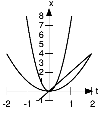
The second derivative can be interpreted as a measure of the curvature of the graph, as shown in Figure 1.11. The graph of the function x=2t is a line, with no curvature. Its first derivative is 2, and its second derivative is zero. The function t^2 has a second derivative of 2, and the more tightly curved function 7t^2 has a bigger second derivative,14.

Figure 1.12

The functions

and

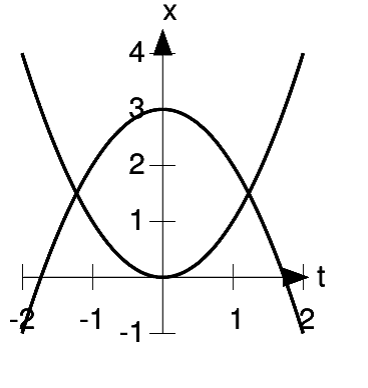
Positive and negative signs of the second derivative indicate concavity. In Figure 1.12, the function t^2 is like a cup with its mouth pointing up. We say that it's "concave up," and this corresponds to its positive second derivative. The function 3-t^2 , with a second derivative less than zero, is concave down. Another way of saying it is that if you're driving along a road shaped like t^2 , going in the direction of increasing , then your steering wheel is turned to the left, whereas on a road shaped like 3-t^2 it's turned to the right.

Figure 1.13 The functions

has an inflection point at

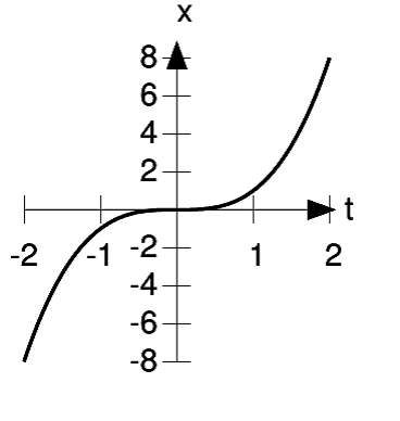
Figure 1.13 shows a third possibility. The function t^3 has a derivative 3t^2 , which equals zero at t=0 . This called a point of inflection. The concavity of the graph is down on the left, up on the right. The inflection point is where it switches from one concavity to the other. In the alternative description in terms of the steering wheel, the inflection point is where your steering wheel is crossing from left to right.

1810 reads

You are here

The second derivative

Example