


***Table 5.1 "A Numerical Example of a Production Function" gives a numerical example of a production function. The first column lists the amount of output that can be produced from the inputs listed in the following columns.
Table 5.1 A Numerical Example of a Production Function
|
Row |
Output |
Capital |
Labor |
Other Inputs |
|
Increasing Capital |
||||
|
A |
100 |
1 |
1 |
100 |
|
B |
126 |
2 |
1 |
100 |
|
C |
144 |
3 |
1 |
100 |
|
D |
159 |
4 |
1 |
100 |
|
Increasing Labor |
||||
|
E |
100 |
1 |
1 |
100 |
|
F |
159 |
1 |
2 |
100 |
|
G |
208 |
1 |
3 |
100 |
|
H |
252 |
1 |
4 |
100 |
|
Increasing Other Inputs |
||||
|
I |
100 |
1 |
1 |
100 |
|
J |
110 |
1 |
1 |
110 |
|
K |
120 |
1 |
1 |
120 |
|
L |
130 |
1 |
1 |
130 |
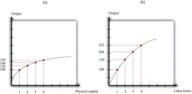
If you compare row A and row B of ***Table 5.1 "A Numerical Example of a Production Function", you can see that an increase in capital (from 1 unit to 2 units) leads to an increase in output (from 100 units to 126 units). Notice that, in these two rows, all other inputs are unchanged. Going from row B to row C, capital increases by another unit, and output increases from 126 to 144. And going from row C to row D, capital increases from 3 to 4 and output increases from 144 to 159. We see that increases in the amount of capital lead to increases in output. In other words, the marginal product of capital is positive.
Similarly, if you compare rows E–H of ***Table 5.1 "A Numerical Example of a Production Function", you can see that the marginal product of labor is positive. As labor increases from 1 to 4 units, and we hold all other inputs fixed, output increases from 100 to 252 units. Finally, rows I to L show that increases in other inputs, holding fixed the amount of capital and labor, likewise leads to an increase in output.
***Figure 5.3 "A Graphical Illustration of the Aggregate Production Function" illustrates the production function from ***Table 5.1 "A Numerical Example of a Production Function". Part (a) shows what happens when we increase capital, holding all other inputs fixed. That is, it illustrates rows A–D of ***Table 5.1 "A Numerical Example of a Production Function". Part (b) shows what happens when we increase labor, holding all other inputs fixed. That is, it illustrates rows E–H of ***Table 5.1 "A Numerical Example of a Production Function".
- 5438 reads
