


The story we have told explains why the economy departs from potential output but says nothing about how (if at all) the economy gets back to potential output. The answer is that prices have a tendency to adjust back toward their equilibrium levels, even if they do not always get there immediately. This is most easily understood by remembering that prices in the economy are, in the end, usually set by firms. When a firm sees a decrease in demand for its product, it does not necessarily decrease its prices immediately. Its decision about what price to choose depends on the prices of its inputs and the prices being set by its competitors. In addition, it depends on not only what those prices are right now but also what the firm expects to happen in the future. Deciding exactly what to do about prices can be a difficult decision for the managers of a firm.
Without analyzing this decision in detail, we can certainly observe that firms often keep prices fixed when demand decreases—at least to begin with. The result looks like that in ***Figure 7.6 "An Inward Shift in Market Demand for Houses". In the face of a prolonged decrease in demand, however, firms will lower prices. Some firms do this relatively quickly; others keep prices unchanged for longer periods. We conclude that prices are sticky; they do not decrease instantly, but they decrease eventually. [***Chapter 10 "Understanding the Fed" provides more detail about the price-adjustment decisions of firms.***] For the economy as a whole, this adjustment of prices is represented by a price-adjustment equation.
Toolkit: Section 16.20 "Price Adjustment"
The difference between potential output and actual output is called the output gap:
output gap = potential real GDP − actual real GDP.
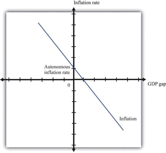
If an economy is in recession, the output gap is positive. If an economy is in a boom, then the output gap is negative. The inflation rate when an economy is at potential output (that is, when the output gap is zero) is called autonomous inflation. The overall inflation rate depends on both autonomous inflation and the output gap, as shown in the price-adjustment equation:
inflation rate = autonomous inflation − inflation sensitivity × output gap.
This equation tells us that there are two reasons for increasing prices.
- Prices increase because autonomous inflation is positive. Even when the economy is at potential output, firms may anticipate that their suppliers or their competitors are likely to increase prices in the future. A natural response is to increase prices, so autonomous inflation is positive.
- Prices increase because the output gap is negative. The output gap matters because, as GDP increases relative to potential, labor and other inputs become scarcer. Firms see increasing costs and choose to set higher prices as a consequence. The “inflation sensitivity” tells us how responsive the inflation rate is to the output gap.
When real GDP is above potential output, there is upward pressure on prices in the economy. The inflation rate exceeds autonomous inflation. By contrast, when real GDP is below potential, there is downward pressure on prices. The inflation rate is below the autonomous inflation rate. The price-adjustment equation is shown in ***Figure 7.14 "Price Adjustment".
We can apply this pricing equation to the Great Depression. Imagine first that autonomous inflation is zero. In this case, prices decrease when output is below potential. From 1929 to 1933, output was surely below potential and, as the equation suggests, this was a period of decreasing prices. After 1933, as the economy rebounded, the increase in the level of economic activity was matched with positive inflation—that is, increasing prices. This turnaround in inflation occurred even though the economy was still operating at a level below potential output. To match this movement in prices, we need to assume that—for some reason that we have not explained—autonomous inflation became positive in this period.
KEY TAKEAWAY
Keynes argued that, at least in the short run, markets were not able to fully coordinate economic activity. His theory gave a prominent role to aggregate spending as a determinant of real GDP.
Given prices, a reduction in spending will lead to a reduction in the income of workers and owners of capital, which will lead to further reductions in spending. This link between income and spending is highlighted by the circular flow of income and underlies the aggregate expenditure model.
The stock market crash in 1929 reduced the wealth of many households, and this could have led them to cut consumption. This reduction in aggregate spending, through the multiplier process, could have led to a large reduction in real GDP.
The reductions in investment in the early 1930s, perhaps coming from instability in the financial system, could lead to a reduction in aggregate spending and, through the multiplier process, a large reduction in real GDP.
***
Checking Your Understanding
Some researchers have suggested that a reduction in US net exports is another possible cause of the Great Depression. Use the aggregate expenditure model to consider the effects of a reduction in net exports. What happens to real GDP?
Suppose autonomous inflation is constant, but real GDP moves around. Would you expect inflation to be procyclical or countercyclical?
- 2075 reads
