


In this chapter, we have discussed the development of E-R diagrams and the foundations for implementing well-constrained relational database models. It is now time to put these two concepts together. This process is referred to as mapping an E-R diagram into a logical database model—in this case a relational data model.
We introduce here a five-step process for specifying relations based on an E-R diagram. Based on the constraints we have discussed in this chapter, we will use this five-step process to develop a well-constrained relational database implementation. Follow along as we map the E-R diagram in Figure 3.13 to the relational database schema in Figure 3.14.
1. Create a separate relational table for each entity.
This a logical starting point when mapping an E-R diagram into a relational database model. It is generally useful first to specify the database schema before proceeding to expansion of the relations to account for specific tuples. Notice that each of the entities in Figure 3.13 has become a relation in Figure 3.14. To complete the schema, however, steps 2 and 3 must also be completed.
2. Determine the primary key for each of the relations. The primary key mustuniquely identify any row within the table.
3. Determine the attributes for each of the entities.
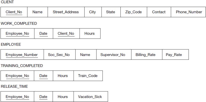
Note in Figure 3.13 that a complete E-R diagram includes specification of all attributes, including the key attribute. This eliminates the need to expend energy on this function during development of the relations. Rather, the focus is on step 2 and now becomes simply a manner of determining how to implement the prescribed key attribute within a relation. With a single attribute specified as the key, this is a very straightforward matching between the key attribute specified in the E-R diagram and the corresponding attribute in the relation (e.g., Employee_Number in the EMPLOYEE entity of Figure 3.13 and the EMPLOYEE relation in Figure 3.14). For a composite key, this is a little trickier—but not much. For a composite key, we can simply break it down into its component subattributes. For instance, in the implementation of the WORK_COMPLETED relation, Employee_No, Date, and Client_No would be three distinct attributes in the relation, but would also be defined as the key via a combination of the three. The completed schema is presented in Figure 3.14. Note the direct mapping between the entities and attributes in the E-R diagram and the relations and attributes respectively in the relational schema.
|
Review Question How is a composite key implemented in a relational database model? |
4. Implement the relationships among the entities. This is accomplished by ensuringthat the primary key in one table also exists as an attribute in every table (entity)for which there is a relationship specified in the entity-relationship diagram.
With the availability of the full E-R diagram, the mapping of the relationships in the diagram with the relationships embedded in the relational schema is again fairly straightforward. References to the key attributes in one entity are captured through the inclusion of a corresponding attribute in the other entity participating in the relationship. However, the dominance of 1:N relationships in our model simplifies this process. Let’s take a quick look at how the different categories of relationships (i.e., cardinality constraints) affect the mapping to a relational schema.
- One-to-many (1:N or N:1) relationships are implemented by including the primary key of the “one” relationship as an attribute in the “many” relationship. This is the situation we have for all of the relationships in Figure 3.13. The linking between these relations in the schema are drawn in Figure 3.15. Note that Client_No in CLIENT and Employee_Number in EMPLOYEE provide the links to WORK_COMPLETED. Similarly, Employee_Number in EMPLOYEE provides links to TRAINING_ COMPLETED and RELEASE_TIME. The recursive relationship with EMPLOYEE is linked using Supervisor_No to identify the correct EMPLOYEE as the supervisor.
|
Review Question What is the difference in implementation of a one-to-many and a one-to-one relationship in a relational database model? |
- One-to-one (1:1) relationships are treated as a one-to-many relationship. But, to implement the one-to-one relationship, we must decide which of the entities is to be the “many” and which is to be the “one.” To do this we might predict which of the “ones” might become a “many” in the future and make that the “many.” If we can’t decide, then either will do. For example, if at present one employee workday was sufficient to complete any client project, then a 1:1 relationship would exist between WORK_COMPLETED and CLIENT. Even in this situation we would still select the Client_No in CLIENT to establish the primary key (see Figure 3.15) in anticipation that in the future a client engagement might require more than one day to complete and more than one employee to complete (i.e., the formation of the many dimension shown in the relationship of Figure 3.13).
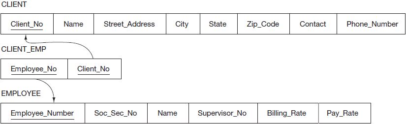
- Many-to-many (M:N) relationships are implemented by creating a new relation whose primary key is a composite of the primary keys of the relations to be linked. In our model we do not have any M:N relationships, but if we had not needed to record the Date and Hours in the WORK_COMPLETED entity, that entity would not have existed. Still, we would then need a relationship between the EMPLOYEE and CLIENT entities which would then be a M:N relationship. This creates problems because our relations cannot store multiple client numbers in a single EMPLOYEE tuple for all clients in which an employee provides services. Similarly, a single CLIENT tuple cannot store multiple employee numbers to record all employees working on an engagement. In that situation, we would have needed to develop a relation to link the EMPLOYEE and CLIENT relations (see Figure 3.16). This new relation would have a composite key consisting of Employee_Number from EMPLOYEE and Client_No from CLIENT—essentially the same as what we currently have with the composite key in the existing relation, WORK_COMPLETED (see Figure 3.15). Note that we wouldn’t combine the columns, but rather just as we have done in the WORK_COMPLETED, TRAINING_COMPLETED, and RELEASE_TIME relations, the individual attributes making up the composite key remain independent in the corresponding relation.
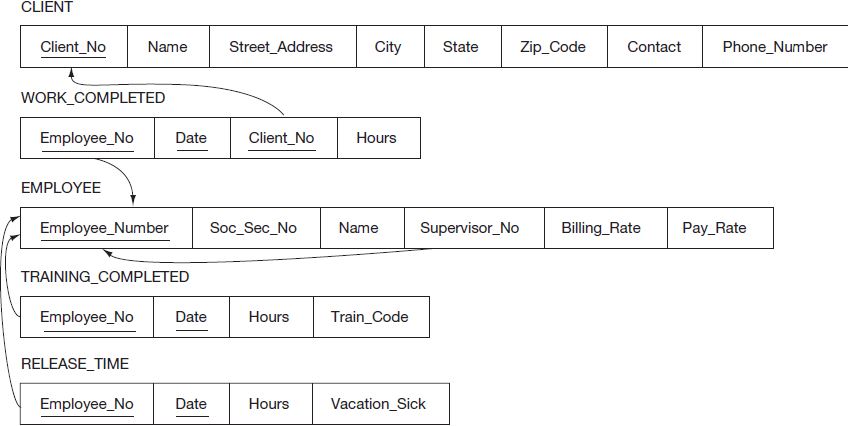

Beyond concerns over meeting the constraint requirements for primary keys, we must also assure adherence to the referential integrity constraints. We identify the referential integrity constraints by locating the corresponding attribute in each relation that is linked via a relationship. We then determine which of the relations contain the tuple that if the reference attribute were deleted or changed would jeopardize the integrity of the database. In Figure 3.15 the referential integrity constraints are represented by arrows, with the destination of the arrow being the attribute requiring control for referential integrity. In other words, the attribute that is pointed to, if changed or deleted, could cause an attribute to have a nonmatching value at the source of the arrow. To ensure referential integrity, constraints should be put in place to assure Employee_Number is not altered or deleted for any EMPLOYEE until the referencing attribute values for the Employee_No attributes in WORK_COMPLETED, TRAINING_COMPLETED, and RELEASE_TIME have first been corrected. Likewise, a similar constraint should be placed on Client_No in CLIENT until Client_No has been corrected in WORK_COMPLETED.
5. Determine the attributes, if any, for each of the relationship tables.
Again, in the extended version of the E-R diagram, the attributes map directly over to the relations. The implementation of the schema is shown in Figure 3.17.
- 61735 reads
